Welcome to the website for my ECE 4160 (Fast Robots) Labs!
I am a junior studying Electrical and Computer Engineering at Cornell University. Looking forward to all the labs we will work on in this course! Hope you enjoy!
Lab 1: Artemis
Objective
Lab 1 was meant to help us get used to using the Arduino IDE and the Artemis Nano.
There was no coding involved since we used the example files provided through the IDE.
Blink Up
The first example toggles the LED between on and off.
Serial Communication
The second example demonstrates UART serial communication between the artemis and my laptop.
When I type something into the serial monitor the input is read by the Artemis and then outputted back into the serial monitor.
AnalogRead
The third example uses AnalogRead for the temperature sensor on the Artemis.
The temperature reading increases from around 33200 to 334000 when I put my finger on the board and decreases from around 334000 to 33200 when I blow on the board.
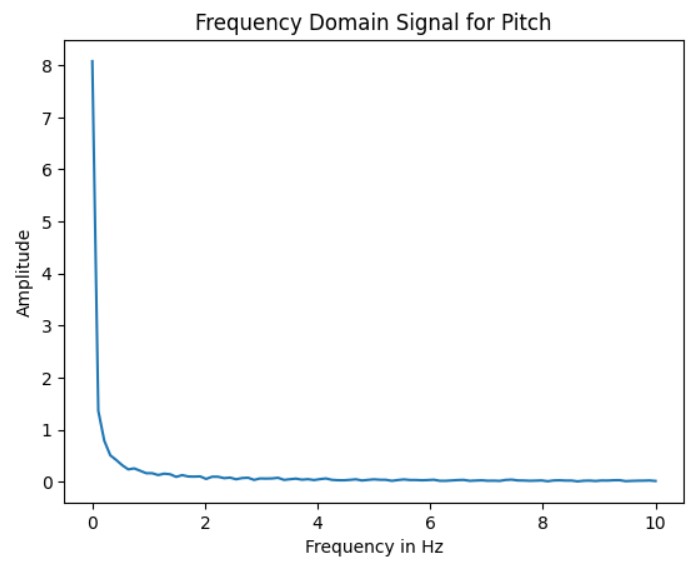
Microphone Output
The final example calculates an FFT and prints the loudest frequency heard by the pulse density microphone on the Artemis.
The frequency increases when I whistle into the microphone.
Lab 2: Bluetooth Communication
Objective
Lab 2's purpose is to establish a bluetooth connection between our computer and the Artemis board.
We will use Jupyter notebook to code in Python and the Arduino IDE for the Artemis.
In future labs we will use bluetooth to communicate between the Artemis and our laptops.
Prelab
Set Up
In order to set up the computer, we had to install Python 3 and pip if they weren't installed already. I also created and activated
a new virtual environment called "FastRbots_ble" which will be used for labs in this course. Within this specific virtual environment
I downloaded the proper packages including 'numpy pyyaml colorama nest_asyncio bleak jupyterlab' so I can run jupyter lab. At this point,
I also downloaded the codebase into my project directory. In addition, to set up the Artemis Board I downloaded the ArdinoBLE library and
ran the sketch ble_arduino.ino to view the MAC address of the artemis board.
Codebase
The code base ble_robot-1.1 contains two sub-directories ble_arduino and ble_python. ble_arduino contains the main ble_arduino.ino
file that we edit in this lab and class definition files. ble_python contains all the files that run in jupyter labs. demo.ipynb is
the main Jupyter Notebook that we can use to run commands and it relies on information from the other files.
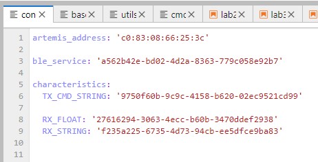
When we run ble_arduino we find out the MAC address of the Artemis which can afterwards be put in connections.yaml. Also, in
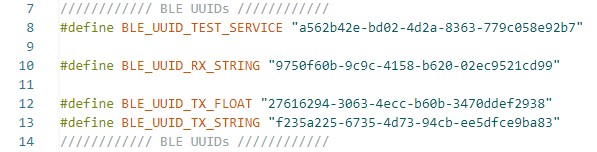
jupyter lab we can randomly generate a uuid which is then copied into connections.yaml and ble_arduino.
In addition, we add a command case to ble_arduino.ino we have to include it in cmd_types.py.
Lab Tasks
Configurations
First I ran the ble_arduino file in arduino to get the mac address of the Artemis board (as done in the prelab) and randomly
generated a uuid in jupyter labs. Afterwards, I updated these values connections.yaml file.
Demo
I ran into a lot of issues when originally running the demo file. My personal laptop runs Windows 11, which at the time of the lab
was not able to properly establish a bluetooth connection between the arduino IDE and bluetooth in jupyter lab. I ended up using the
lab computers but it was to no avail. During the lab section it seemed other students were connecting to the board by accident while
I could not connect to it.
After a week of testing things out, TA Alex posted step by step instructions for how to set up bluetooth communication on Windows 11
It was very helpful and I was finally able to start making progress on the lab.
This is a video running through the Demo File:
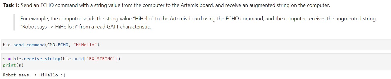
Task 1: ECHO
The ECHO command sends a specific string to the Artemis board and the Artemis sends back the string to the computer. This is done
with interactions between a jupter notebook file and the arduino IDE. In juptyer I called ble.send_command(CMD.COMMAND, "some string")
to send the command to Arduino's switch-case statements. I almost forgot to add the command to the CommandTypes enum and the cmd.types.py file.
Task 2: GET_TIME_MILLIS
This task also used the ble.send_command() and ble.receive_string() to send and receive information bewteen the computer and Artemis.
I used millis() to get the current time in milliseconds and appended it to the string characteristic.
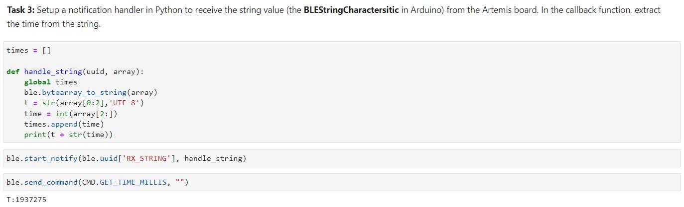
Task 3: Notification Handler
I set up a notification handler and callback function to extract the time from the string sent from the Artemis command GET_TIME_MILLIS
to the laptop. In order to extract the string, I had to first process the data. Since I knew the format of the string being received,
it was easy to splice the string depending on where there were colons and add all the times to an array of times.
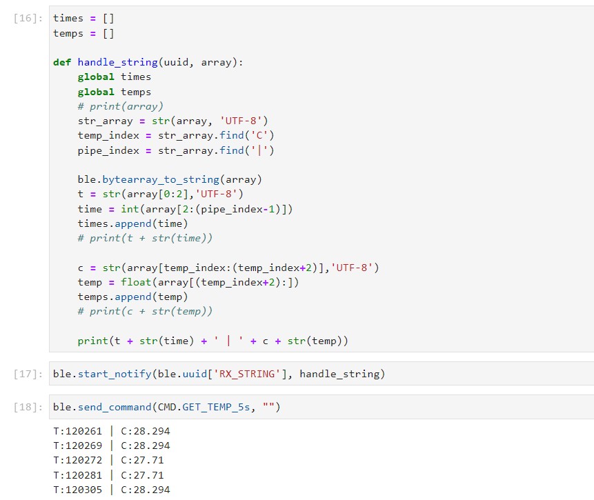
Task 4: GET_TEMP_5s
I added another case statement in the ble_arduino.ino file which sends an array of timestamped temperature readings that were taken
once per second for five seconds. I followed the example temperature file from Lab 1 as a guide for how to read the temperature in
Celsius and used the GET_TIME_MILLIS case as the base code before adding temperature.
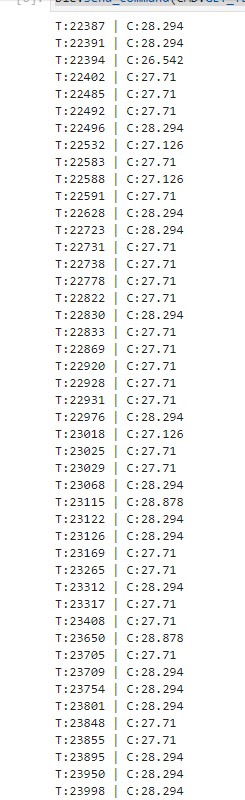
Task 5: GET_TEMP_5s_RAPID
The notification handler for GET_TEMP_5s_RAPID remained the same from the previous task. The difference was in how we loop to collect
a series of data points, for example, checking the time we started taking measurements and subtracting it by the current time to see
if the different was less than or equal to 5000 milliseconds (5 seconds). There were over 50 reading that were taken.
Task 6: Limitations
The Artemis has 384 kB of RAM and we are asked to discuss the limitations of how much data we can store to send without running
out of memory in the form of "5 seconds of 16-bit values taken at 150 Hz".
Since we are transmitting 16-bit values at 150 Hz, we are transmitting 300 bytes per second or 1500 bytes every 5 seconds.
If we divide our total amount of RAM 384 kB by 1500 bytes every 5 seconds, we can transmit 256 5-second intervals of data
before running out of memory.
Resources
Thank you Olive and Alex for the Ed Discussion posts on how to get bluetooth connection working on Windows 11!
Also, I looked at classmates websites such as Tiffany Guo, Liam Kain, Ignacio Romo, Michael Crum, and Samantha Cole.
Lab 3: TOF
Objective
Lab 3's purpose is to set up communication between the Artemis and time of flight sensors. After learning how to read
data from the time of flight sensors, we build off of lab 2 to quickly send data to our computers.
Prelab
I2C Sensor Address
The default address of the TOF sensor is 0x52. This informaton can be found on the VL53L0X datasheet.
Using 2 ToF Sensors
There are two approaches for using two TOF Sensors in parallel because they both have the same address. The first option is to
turn off one TOF sensor during set-up, changing the address of the other sensor, and then turning the TOF sensor back on. At this
point, both TOF sensors would have different addresses and you can read data from both at the same time. The second option is to keep
both TOF sensors with the same address but alternate between turning on and off one sensor when you want to read data from the other one.
An issue that may arise later on is the delay when waiting for the sensors to start back up.
I decided to go with the first option because I don't want to deal with delays later on when my robot is navigating and doing stunts. In addition,
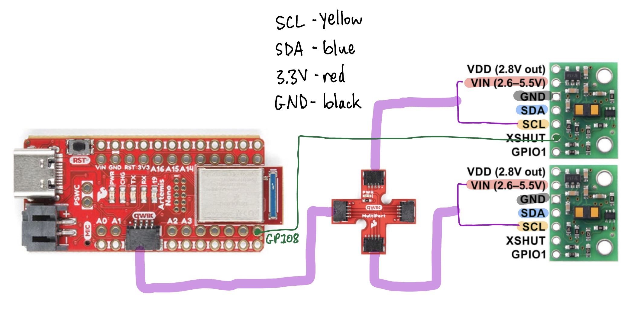
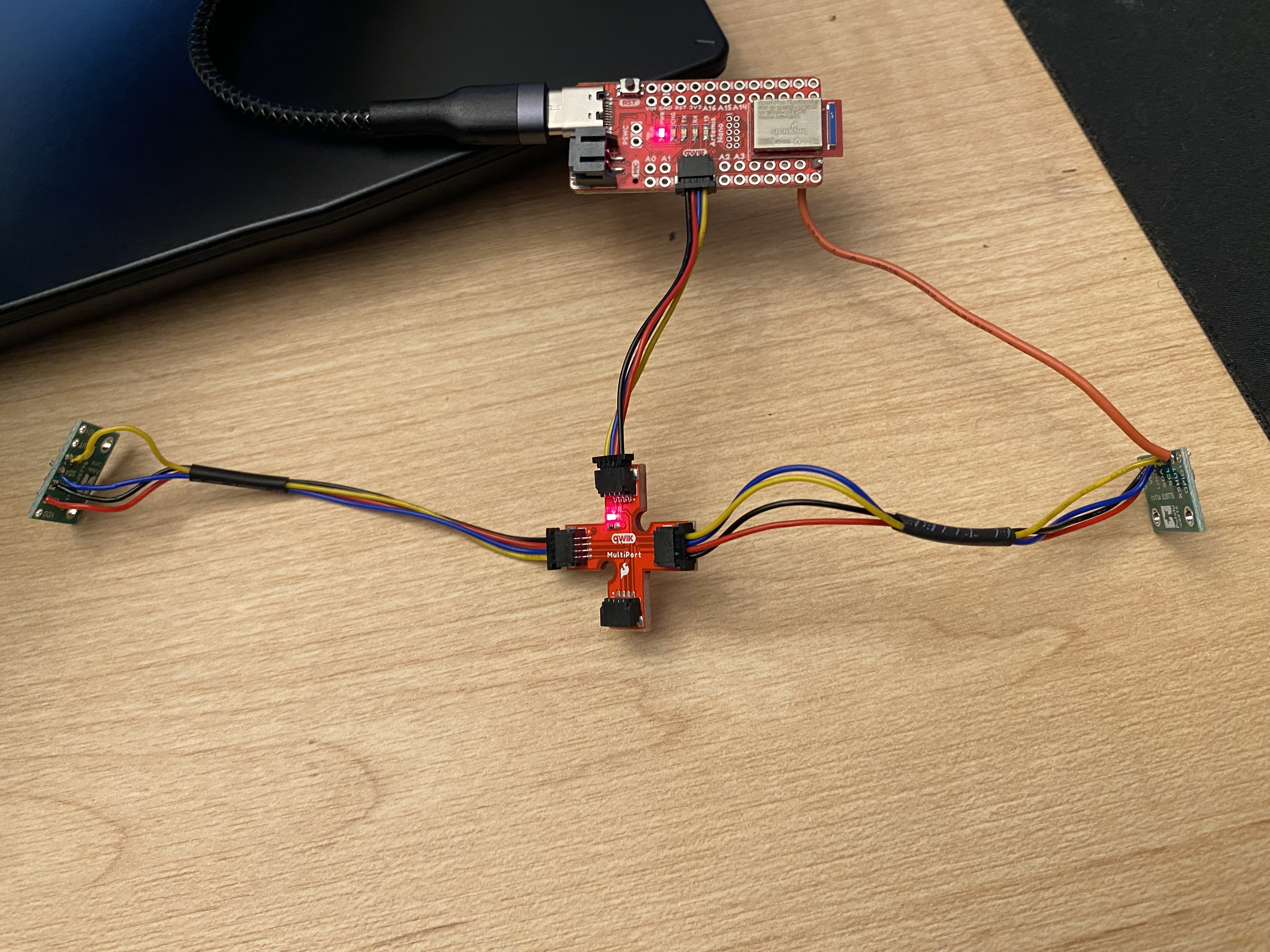
I only have to solder the XSHUT pin on one of the TOF sensors to a GPIO pin (I chose GPIO 8) on the Artemis.
Placement of Sensors
There are many different options for how to place the sensors on the robot. The first option is having a sensor on the left and right sides of
the robot however this means the robot will be unable to detect objects that are in front of it. The second option is having a sensor on the
front and another sensor on one side. This allows for the robot to see in front, but it can cause issues of the robot is coming close to an
obstacle on the side without the sensor. The third option is to place both sensors at an angle on the front of the robot. This allow for the
sensors to see both in front and to the sides. One thing to think about is how to process that data to give reliable and useful information
if the sensors are at an angle.
Wire Diagram
Lab Tasks
ToF Sensor connected to QWIIC Breakout Board
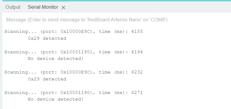
Artemis scanning for I2C Devices
As mentioned in the prelab, the default address of the TOF sensor is 0x52. However, when scanning for I2C devices the address is
0x29 which is equal to 0x52 bitshifted to the right. The least significant bit is used to determine if the device is read/written.
Sensor data with chosen method
The TOF sensor we are using has two measure modes. The short distance mode is used by default which measures up to 1.3 m. The long
distance mode can measure up to 4 m. For the purpose of this lab, I continued to use the default setting. It might be good to use
the long distance mode for the actual robot since it will be moving at a faster speed and needs enough time to react to obstacles
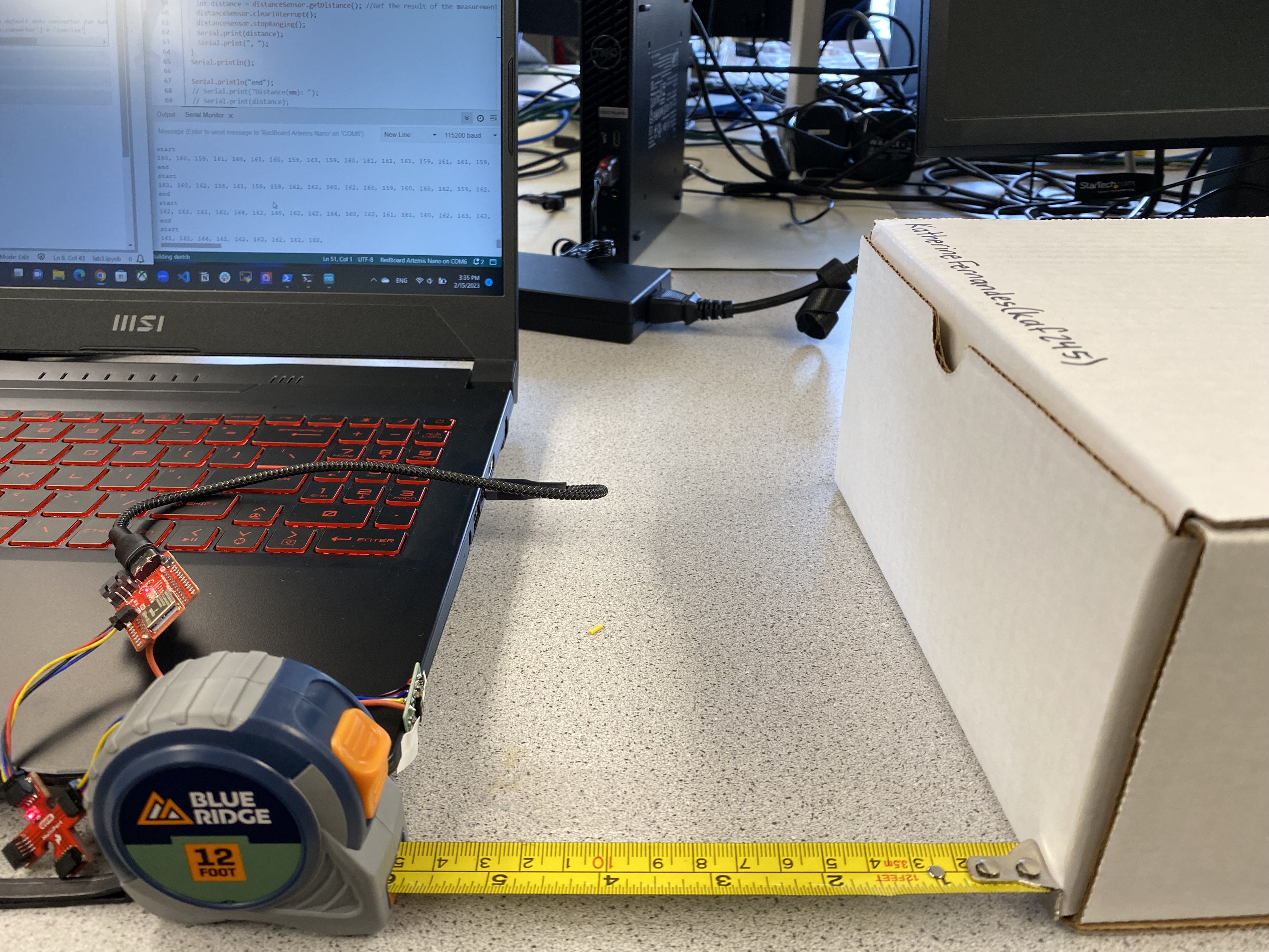
Example setup for measuring 150 mm:
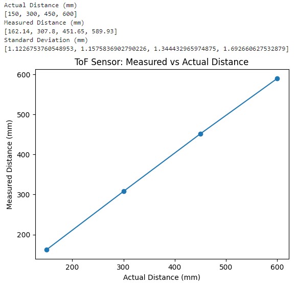
I calculated the mean and standard deviation of 100 measurements for 150 mm, 300 mm, 450 mm, and 600 mm. Below is the plot with
the actual value on the x-axis and the measured values on the y-axis:
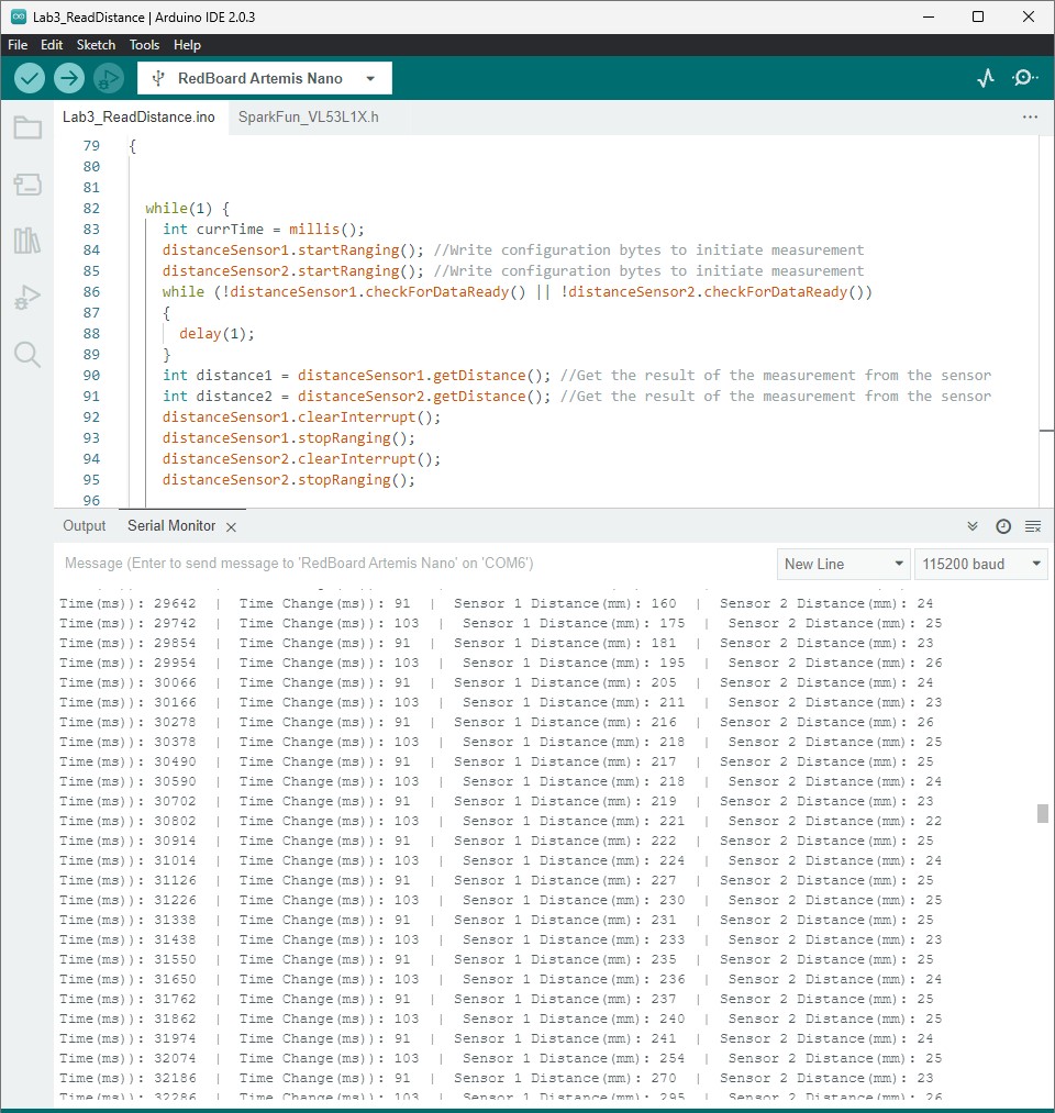
2 ToF Sensors in Parallel
As described in the prelab, I decided to change the address of one of the sensors to 0x54 to use both sensors in parallel.
Below is a screenshot of both sensors measuring different distances.
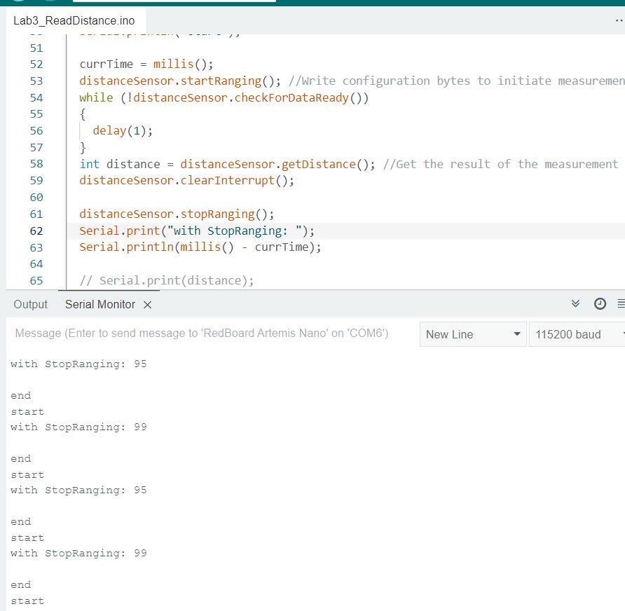
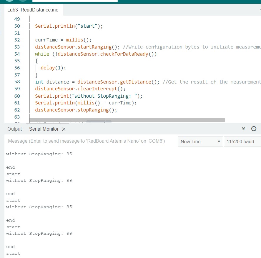
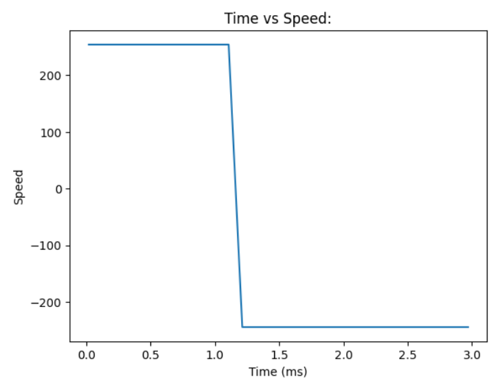
ToF Sensor Speed
Timing with Stop Ranging is about 95-99 ms
Timing without Stop Ranging is about 95-99 ms
Timing for just reading is about 2 ms
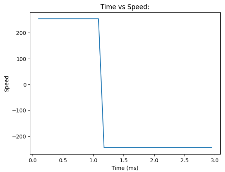
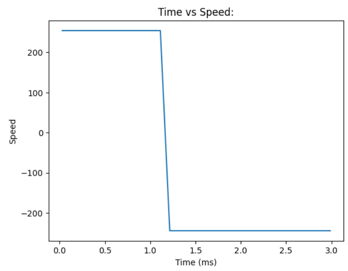
Time vs Distance
I edited some of the Lab 2 code to record time-stamped ToF data for a set period of time and send it to my computer using Bluetooth.
By using the callback function from lab 2 I was able to extract the data from the given string and plot it on a graph. The graph
shows the distance measurements when both sensors collect data at the same time.
Resources
I looked at classmates websites such as Tiffany Guo, Liam Kain, Ignacio Romo, Michael Crum, and Samantha Cole.
Lab 4: IMU
Objective
Lab 4's purpose is to familiarize oursevles with reading data from the IMU and understanding what is means. Also, run the Artemis with
the sensors from a battery. The final task is to record a stunt of the RC car and graph the IMU and TOF data.
Lab Tasks
Set up the IMU
In order to set up the IMU, we had to install the SParkFun 9DOF IMU Breakout - ICM 20948 - Arduino library.
In the setup, AD0_VAL which represents the last but of the IMU's I2C address.
AD0_VAL is set to 1 by default, but when the ADR jumper on the IMU is closed, it should be 0. In our case, the value is 1 because the ADR jumper is not closed.
The basics example was run to see if IMU's accelerometer and gyroscope were properly measuring data. Below is a video of the example code running.
In order to know that the board is running, I set the blue LED on the Artemis board to toggle on and off three times on start up.
Accelerometer
During lecture we went over the equations for pitch (rotation around the y-axis) and roll (rotation around the x-axis):
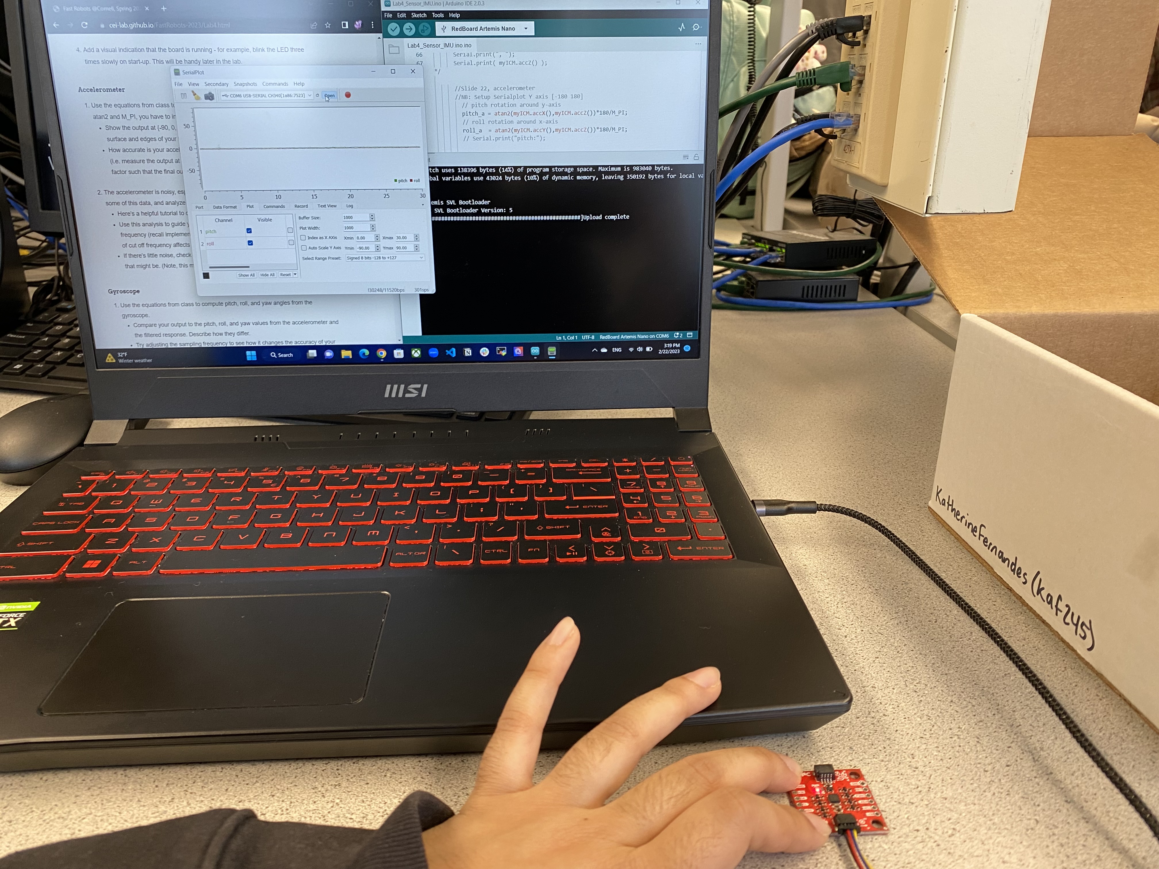
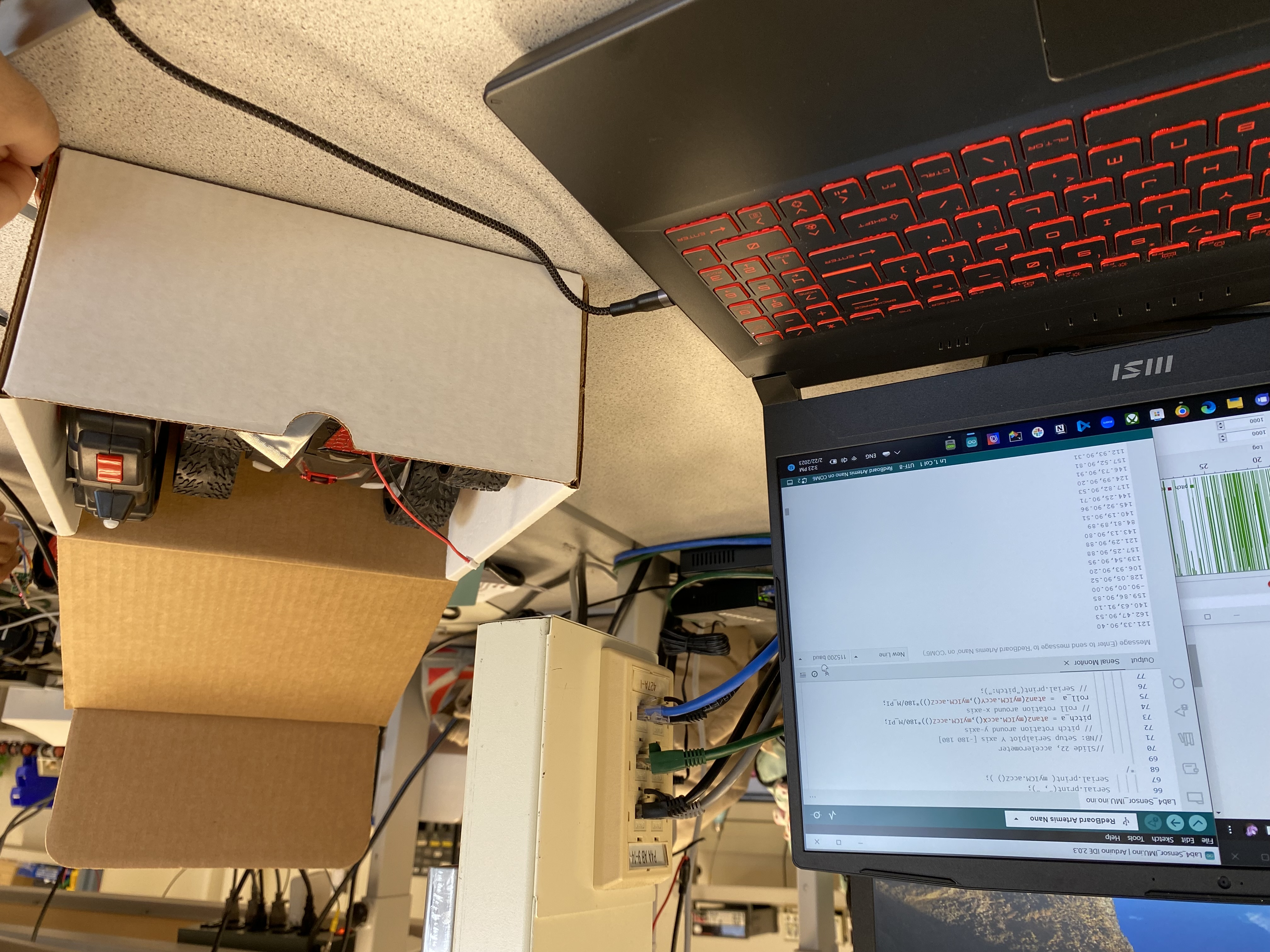
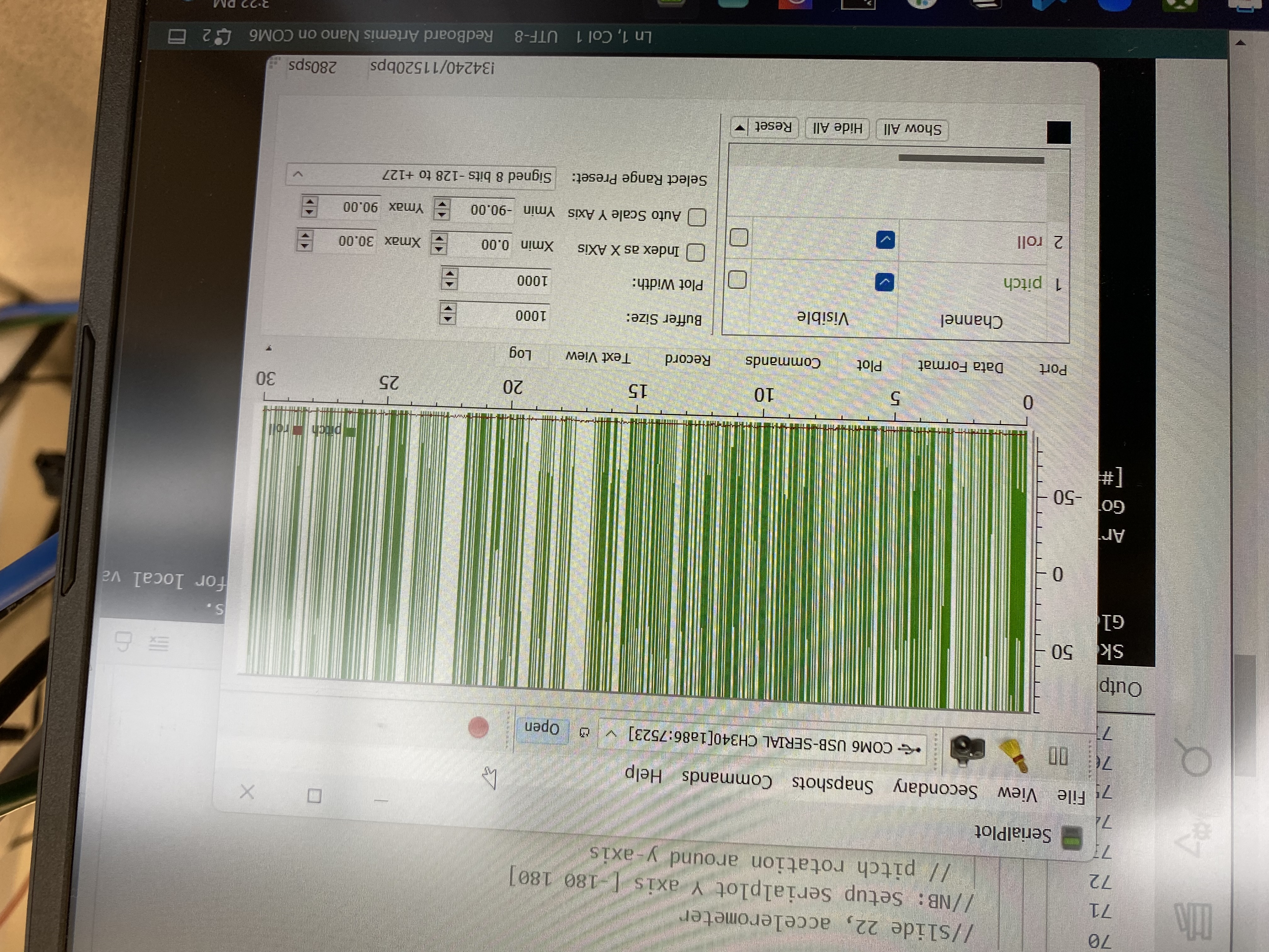
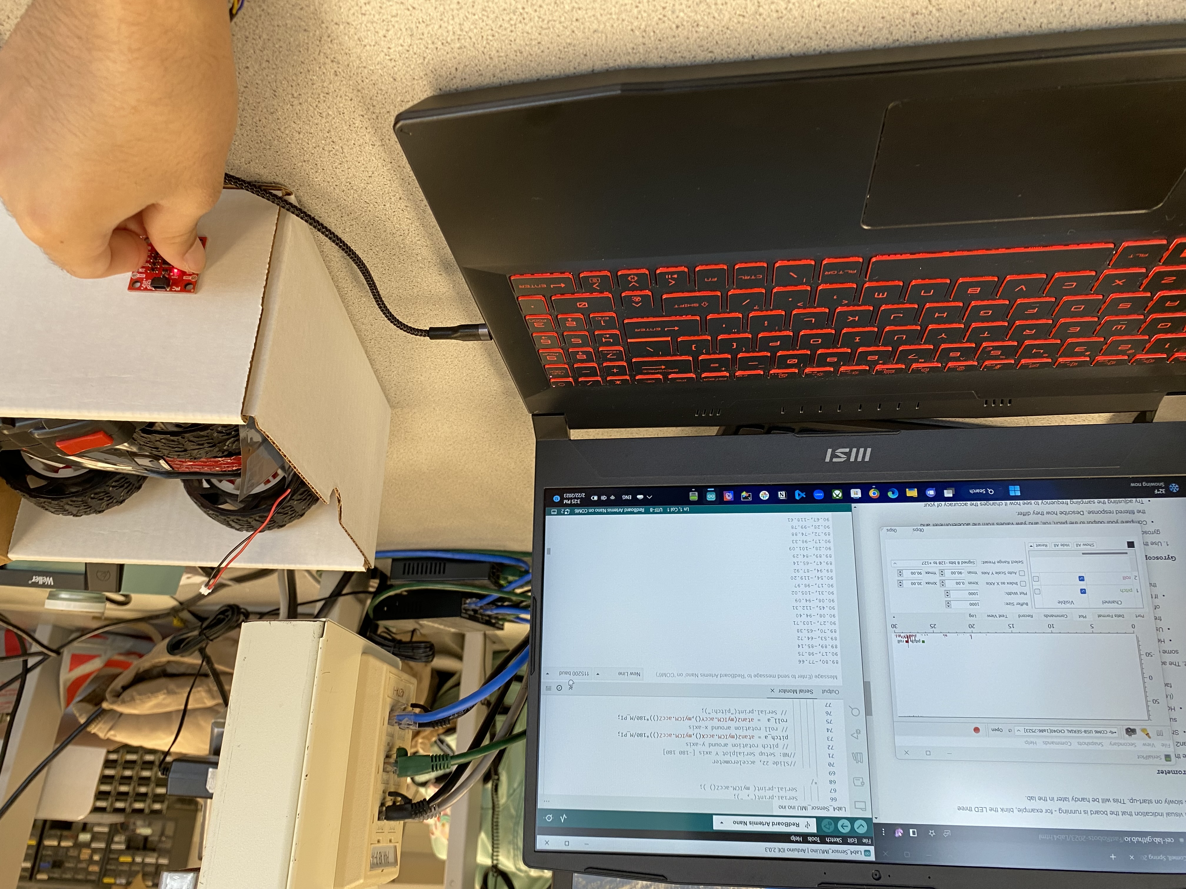
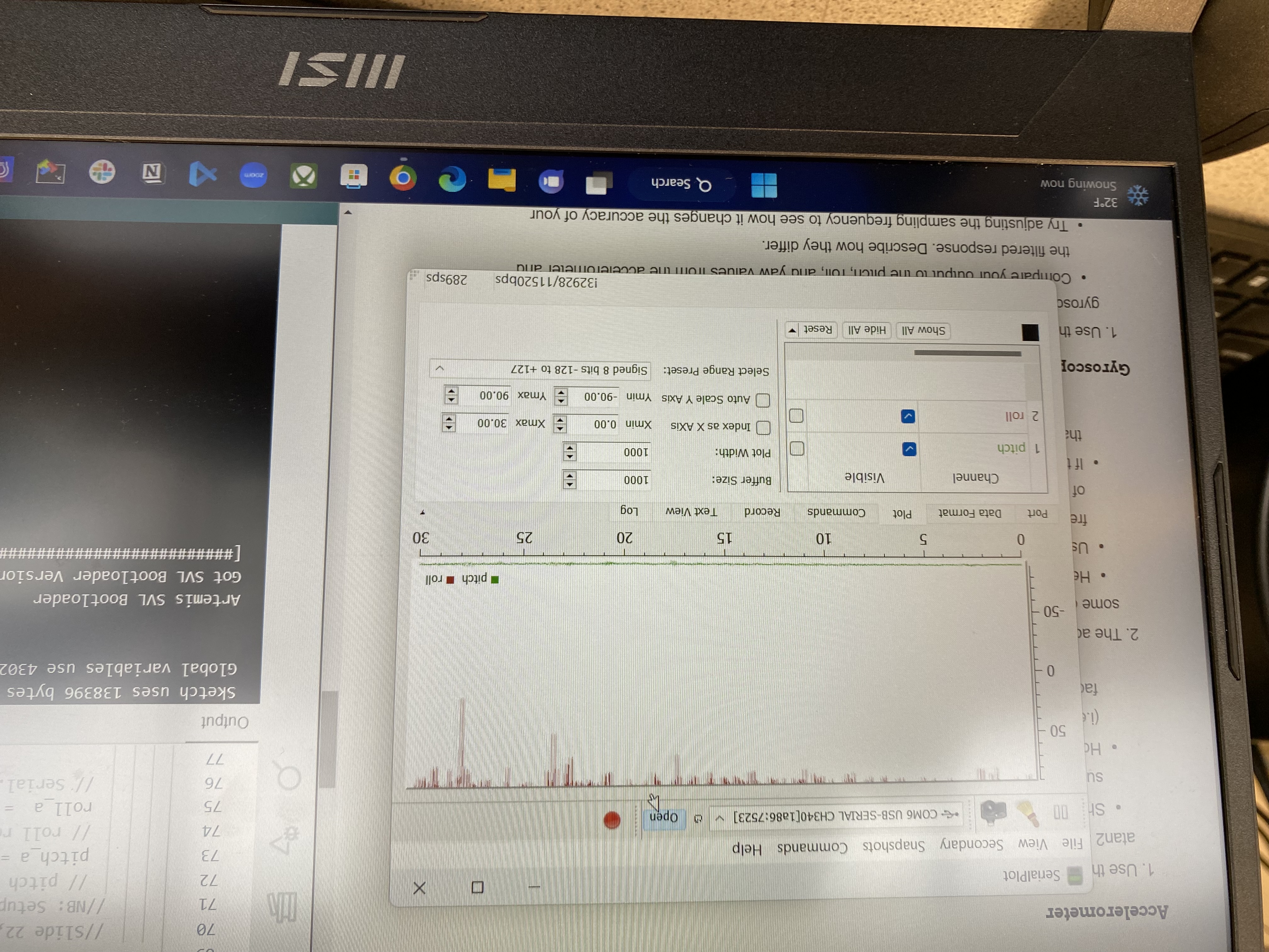
I made a separate arduino file that initializes the IMU to collect data and print into the serial monitor in a specific format
of "data1,data2" so I could plot the data in the Serial Plotter which receive the data from the same COM the Artemis is connect to.
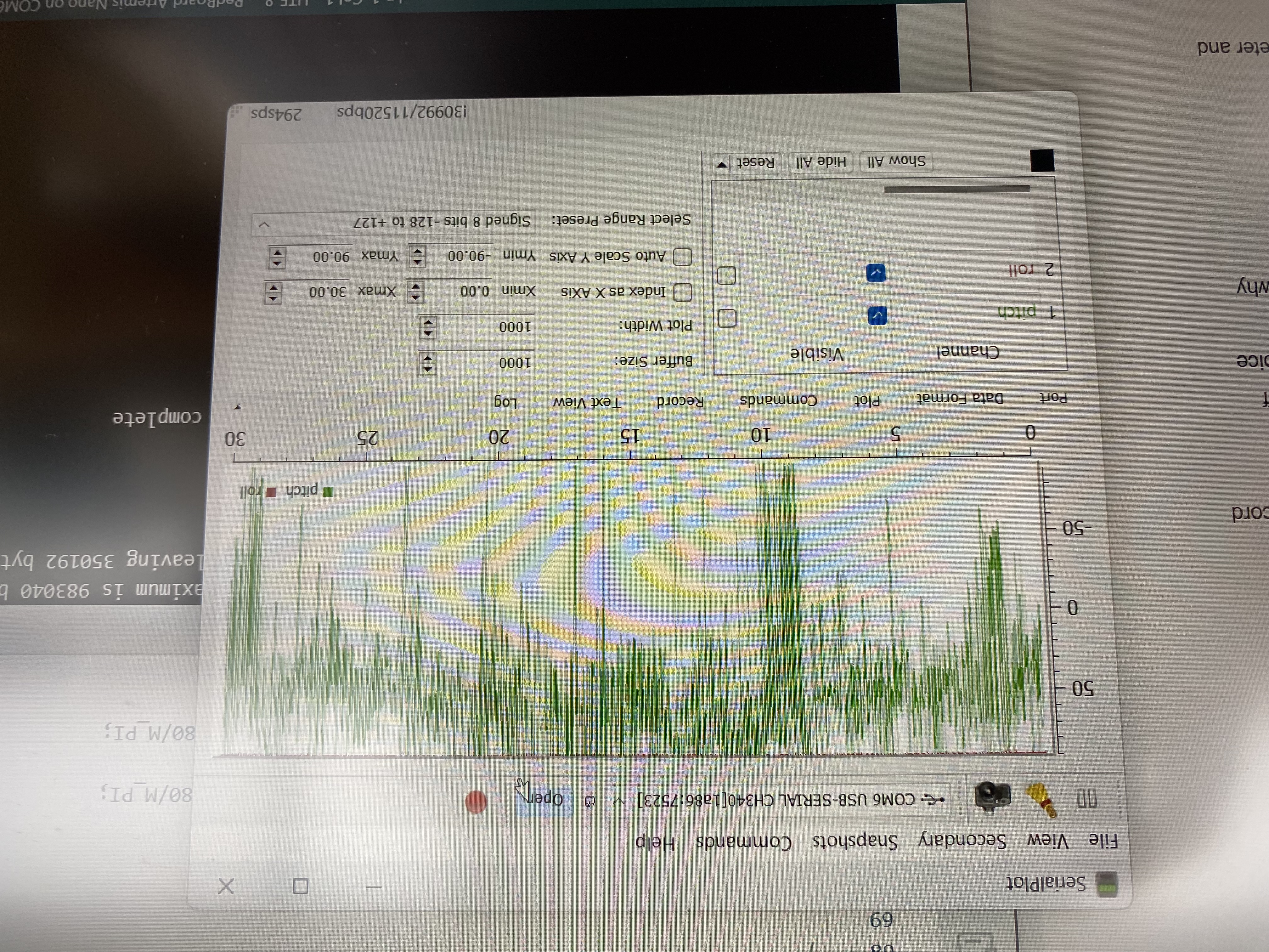
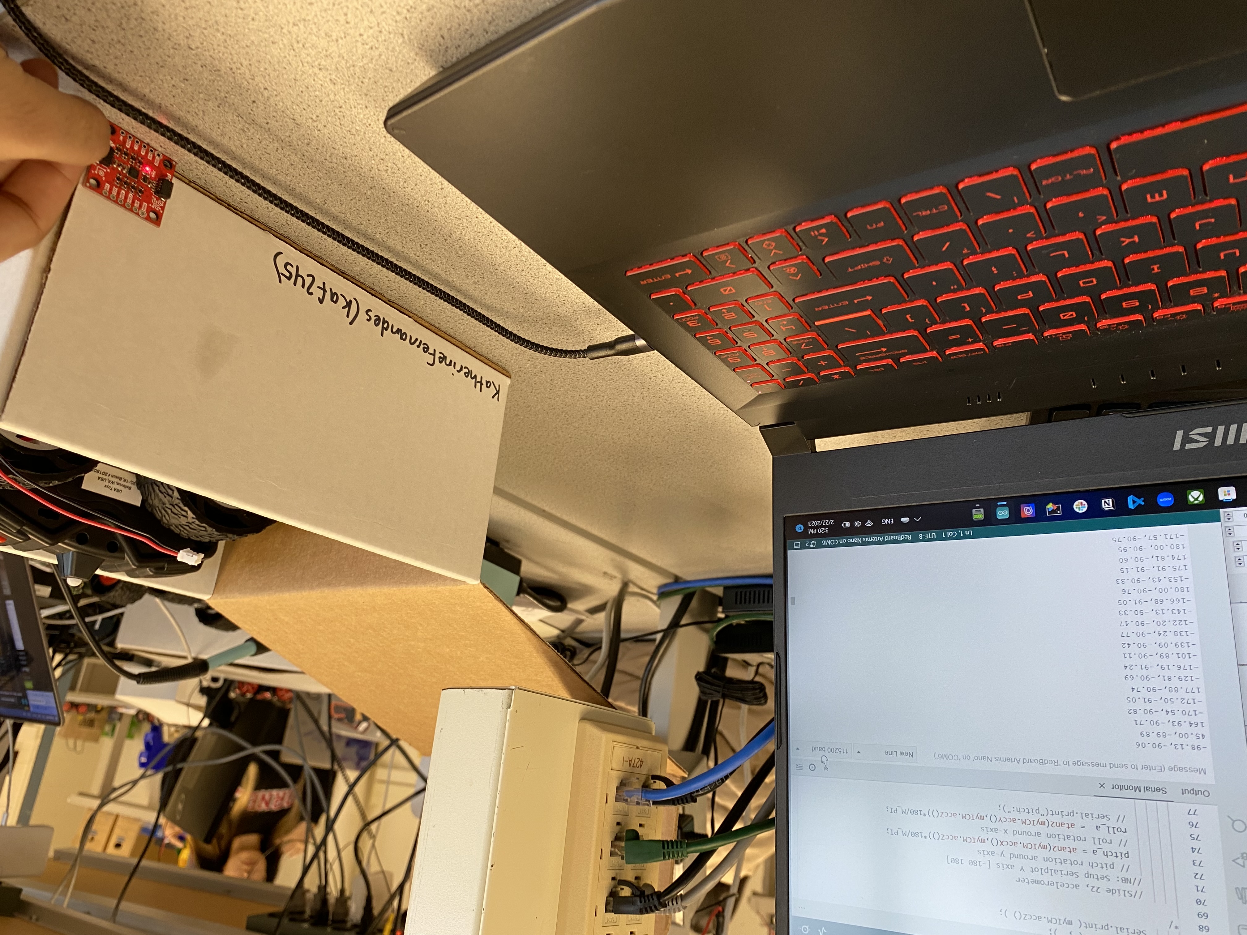
First, I used my lab box as a guide to make sure I was tilting the IMU by +/- 90 degrees about both the x- and y-axis. The images
below show the different orientations with the pitch and roll printed in the Serial Monitor and displayed in the Serial Plotter.
For the serial monitor, it is printed as pitch,roll and for the Serial Plotter the pitch is in green and the roll is in red.
Pitch (green) and Roll (red): 0 degrees
Roll (red) +90 degrees
Roll (red) -90 degrees
Pitch (green) +90 degrees
Pitch (green) -90 degrees
Aftwerwards, I took a video of rotating the IMU in different directions and plotted the pitch and roll in the Serial Plotter.
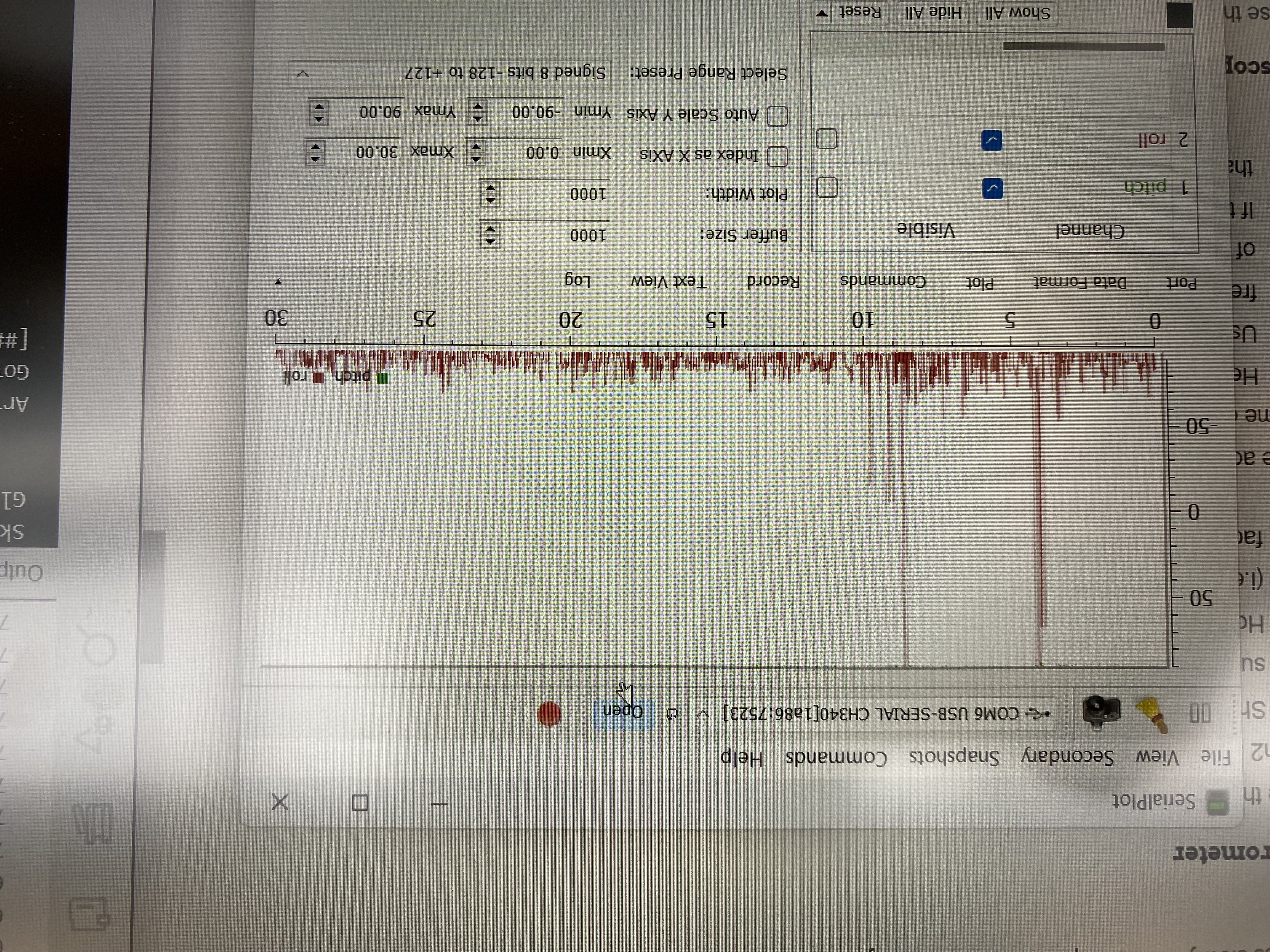
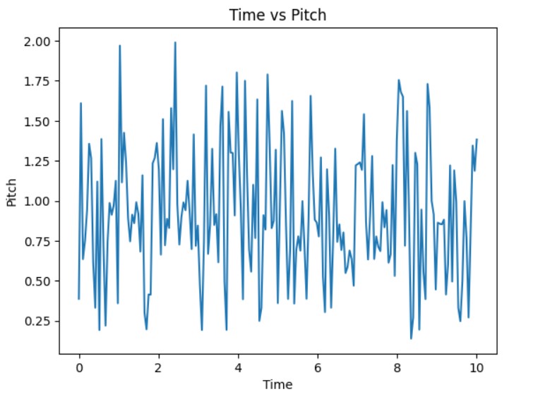
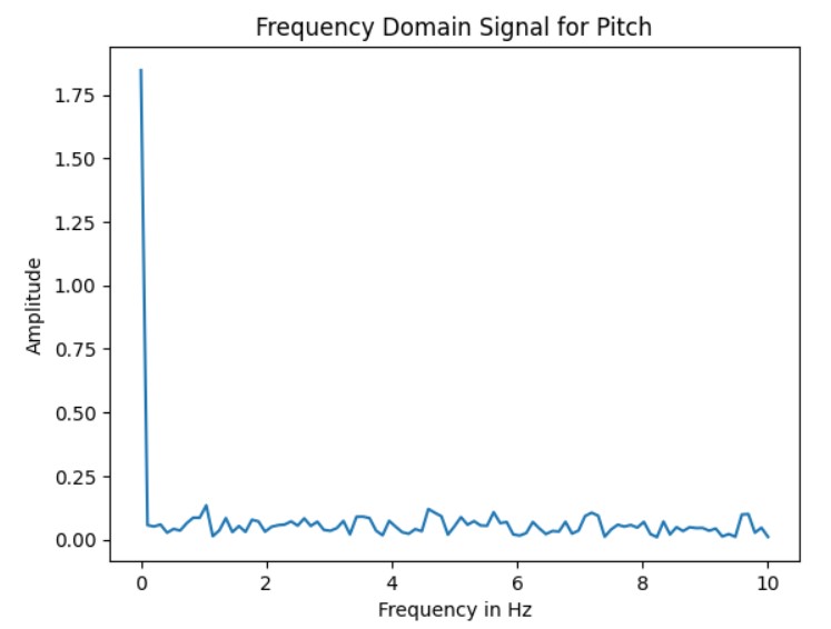
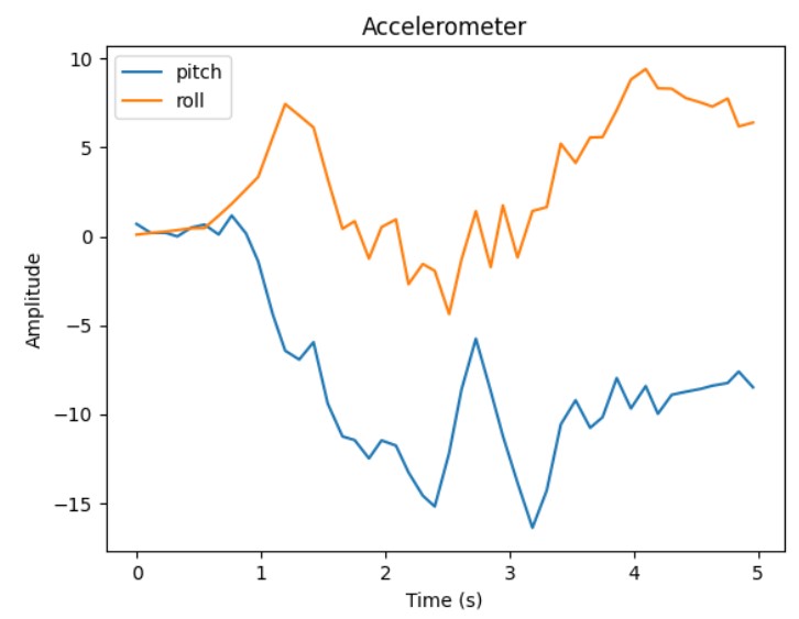
When running the RC car in its proximity there is extra noise in the accelerometer data. I recorded some of this data
by running the car near the accelerometer. I send this data from the Artemis to Python using a modified version of the
bluetooth code from lab 2. In Jupyter lab, I took the FFT of the pitch and the roll which was slightly noisy. In order
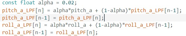
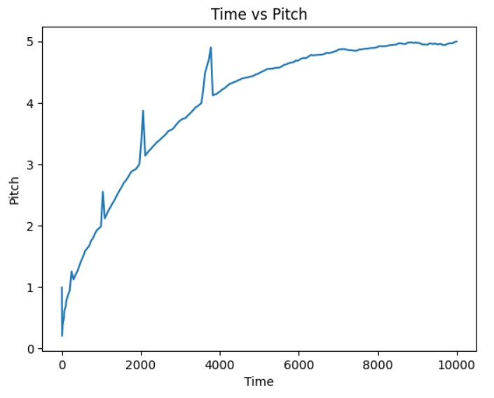
to eliminate some of this noise, I implemented a low pass filter for both the pitch and roll.
Without Low Pass Filter:
With Low Pass Filter:
Gyroscope
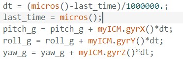
In lecture we also discussed the equations to compute the pitch, roll, and yaw using the gyroscope data:
As shown in the video values output from the gyroscope are much more steady than the outputs from the accelerometer.
However, overtime the offset accumulates to have a large magnitude.
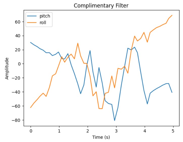
In order to have both the steady nature of the gyroscope and the accuracy of the accelerometer I
implemented a complimentary filter to compute an estimated pitch and roll using information from
both the gyroscope and accelerometer.
Sample Data
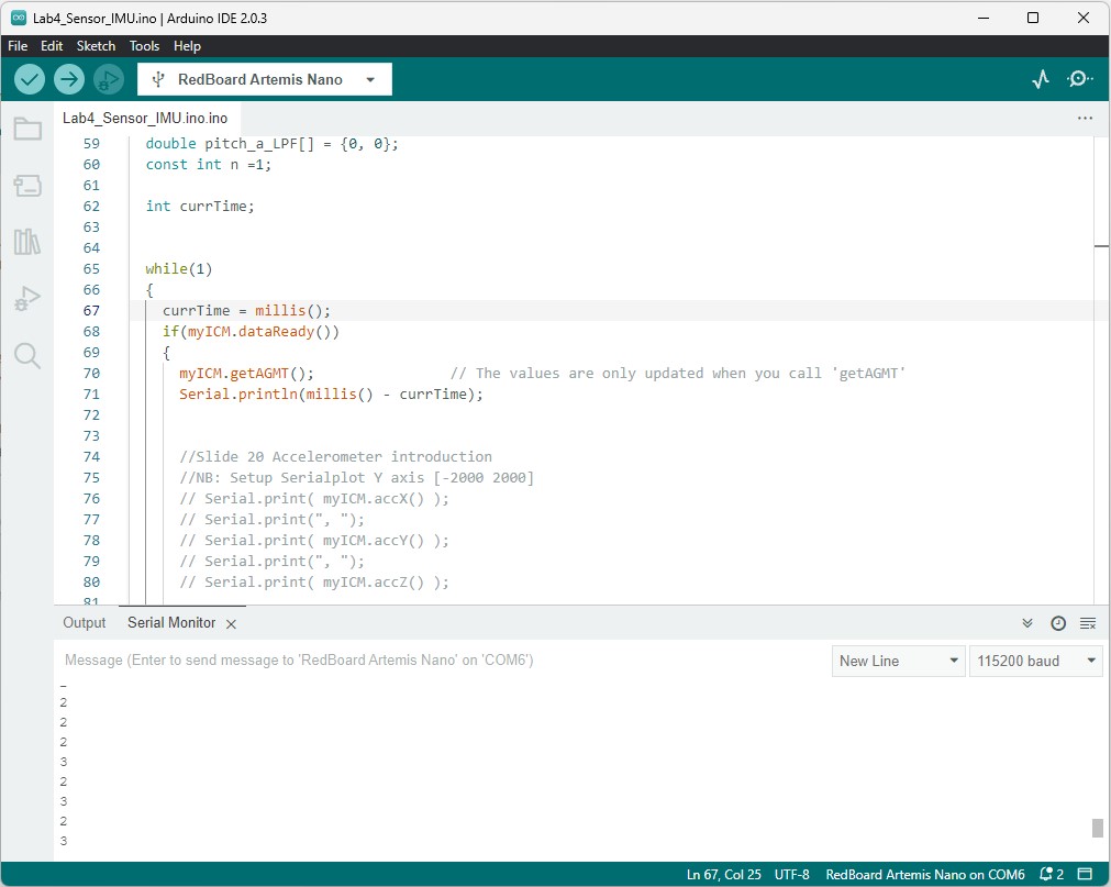
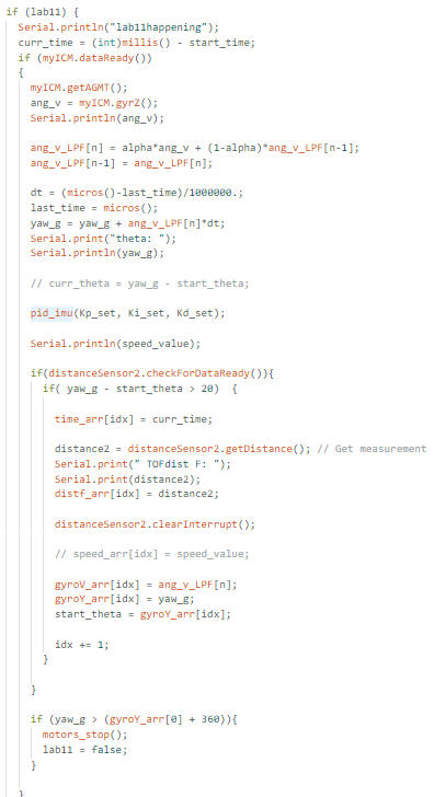
Similar to what was done in lab3, I checked each iteration of the loop for if the IMU was ready.
I removed any of the extra print statements and delays and found the difference in time from before
and after checking if the IMU is ready using myICM.dataReady() and after calling myICM.getAGMT() which updates the values of the IMU.
As shown in the screenshot, I can sample data as fast as 2-3 milliseconds.
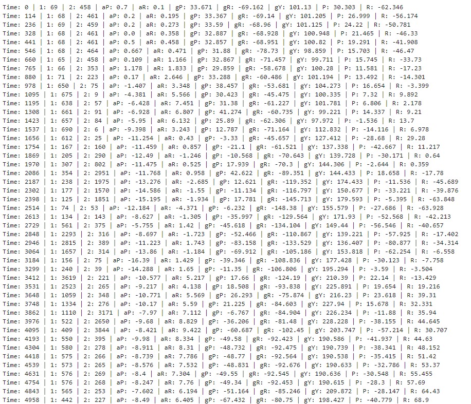
I integrated my code from Lab 3 to collect both ToF and IMU data and sent it over bluetooth
to my laptop. It could collect the data for 5s and then graphed the data using matplot.
I ended up using one big array formatted as a string to store the ToF, accelerometer, and
gyroscope data before sending it to Jupyter Lab. In Jupyter Lab, the string was received and
the data was extracted and separated it into smaller arrays.
Cut the Coord
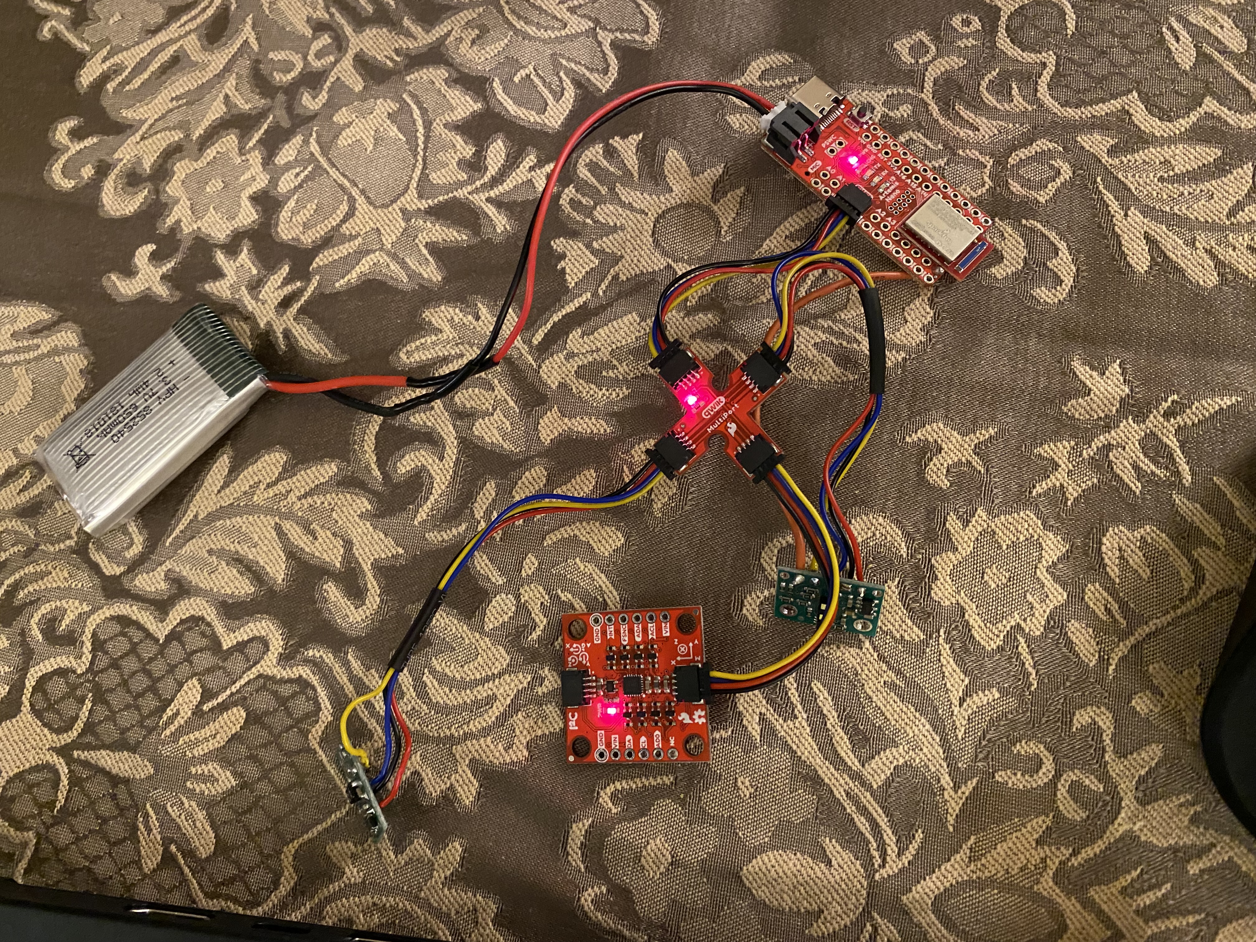
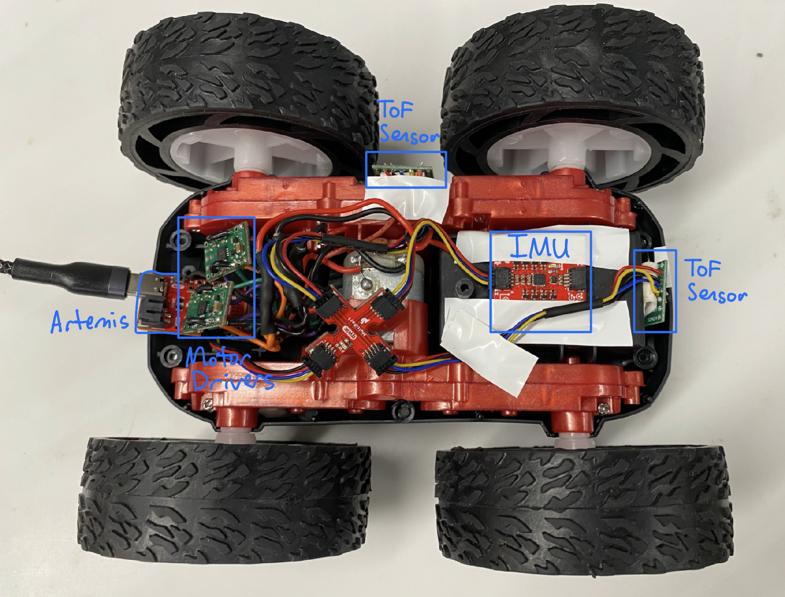
We have two different batteries. One 3.7V 850mAh for the motors and one 3.7V 650mAh for the Artemis and sensors.
We are using the 850mAh one for the motors because the motors will use up the battery much faster. In addition, for the later labs we will be using motor drivers to control the
RC car's motors which will require more current. On the otherhand, the Artemis uses the 650mAh battery since it does
not require as much power.
In order to connect the 650mAh battery to the Artemis, I soldered the cables to the JST connector and used heat shrink
to cover the job.
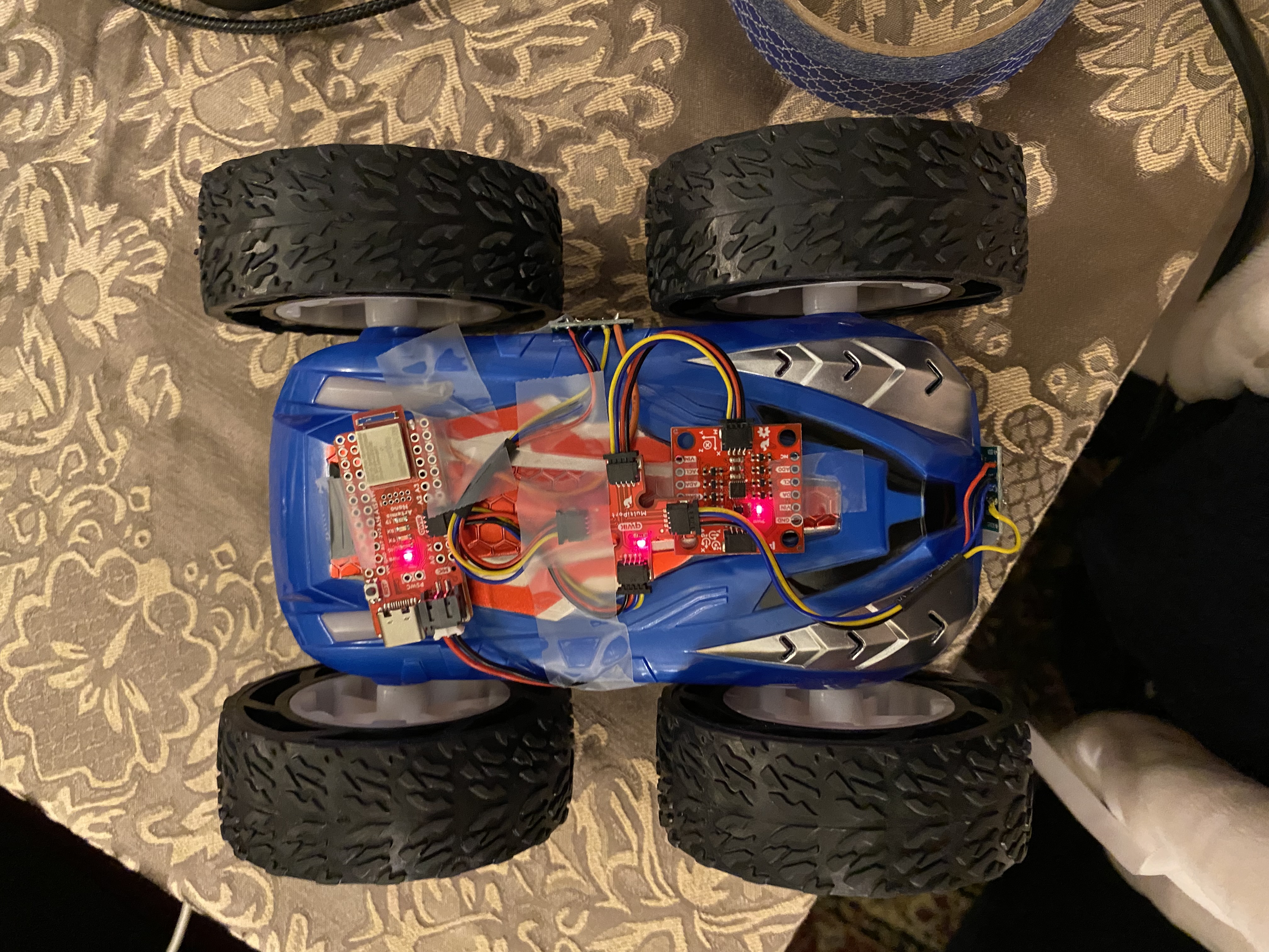
Record a Stunt
I plugged in the 850mAh battery to the RC car and drove it around the hallway for a little while as shown in the video.
Aftwards I attached the 650mAh to the Artemis and everything to the RC car.
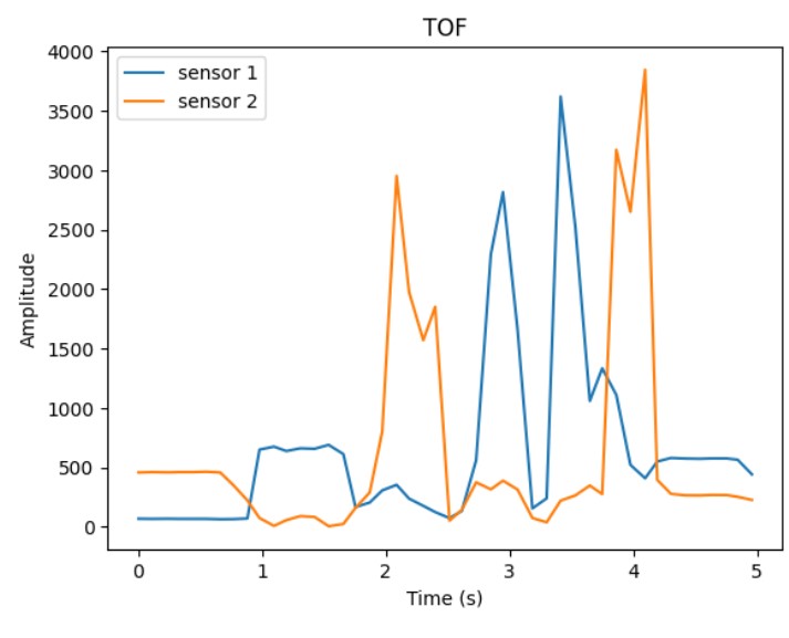
I put one TOF sensor on the left side of the car and the other one on the front of the car. I mounted the IMU, Artemis,
and QWIIC breakout board to one side of the car and the battery to the other side of the car.
I was able to test and see that the bluetooth successfully connected and data collected and sent to my laptop to analyze and graph the outputs
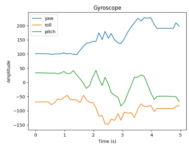
from the accelerometer, gyroscope, and TOF sensors.
Below is a video of the stunt with everything attached and collecting data:
Here are the graphs of the data collected during the stunt:
Resources
I looked at classmates websites such as Tiffany Guo, Zin Tun, Jueun Kwon, Liam Kain, Ignacio Romo, and Michael Crum.
Lab 5: Motor Driver and Open Loop Control
Objective
Lab 5's purpose is to shift from manual to open loop control of the car. This is done
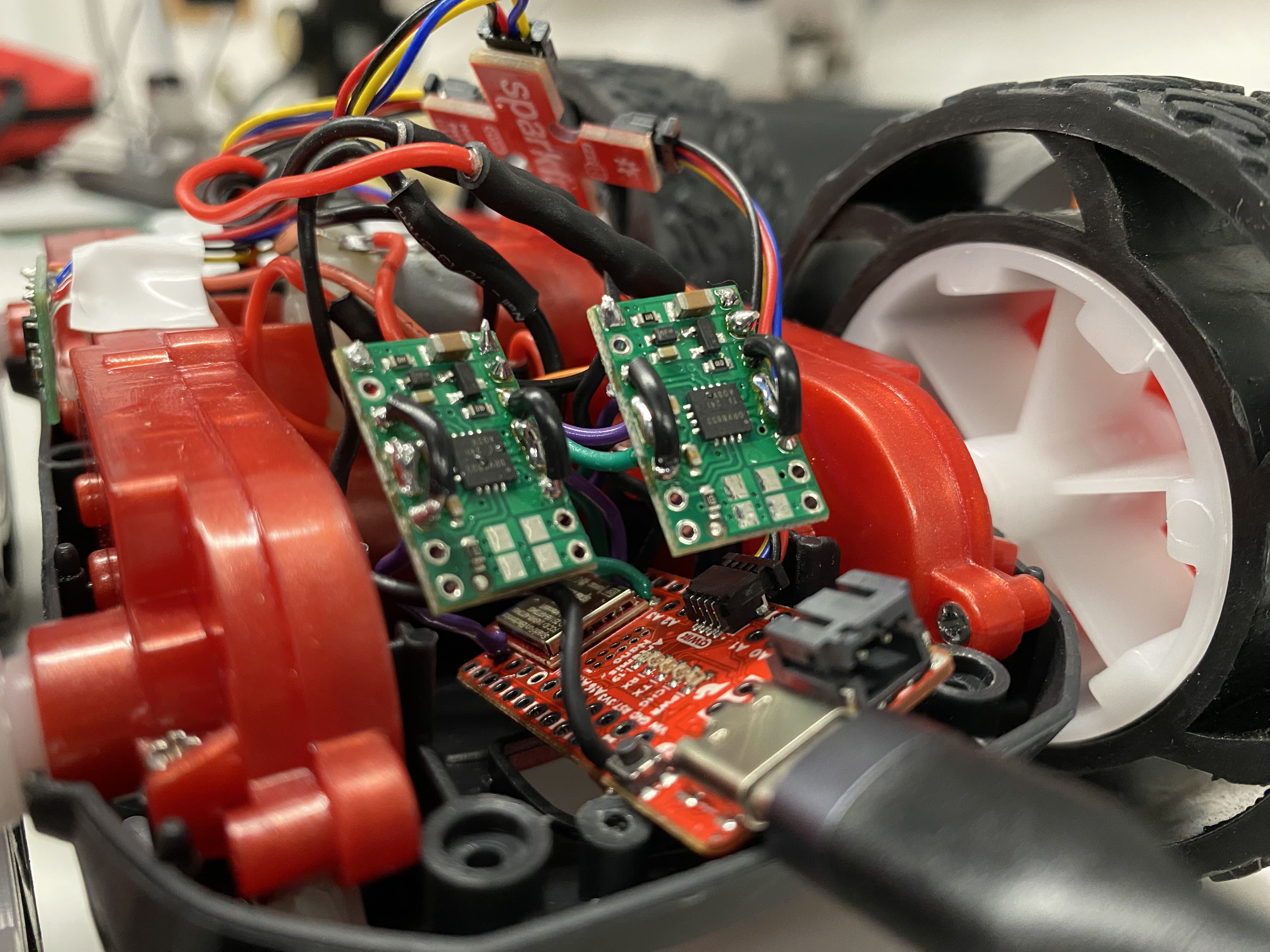
by opening the RC car and replacing the PCB with the Artemis and dual motor drivers.
Prelab
Diagram
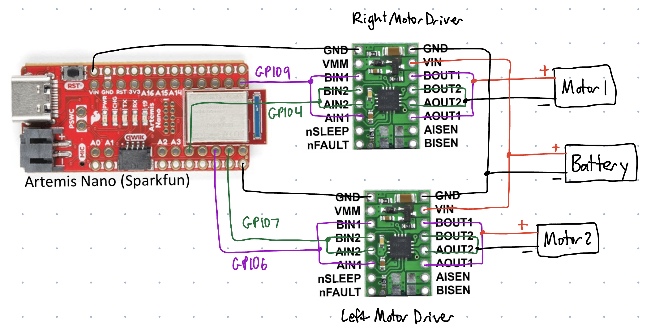
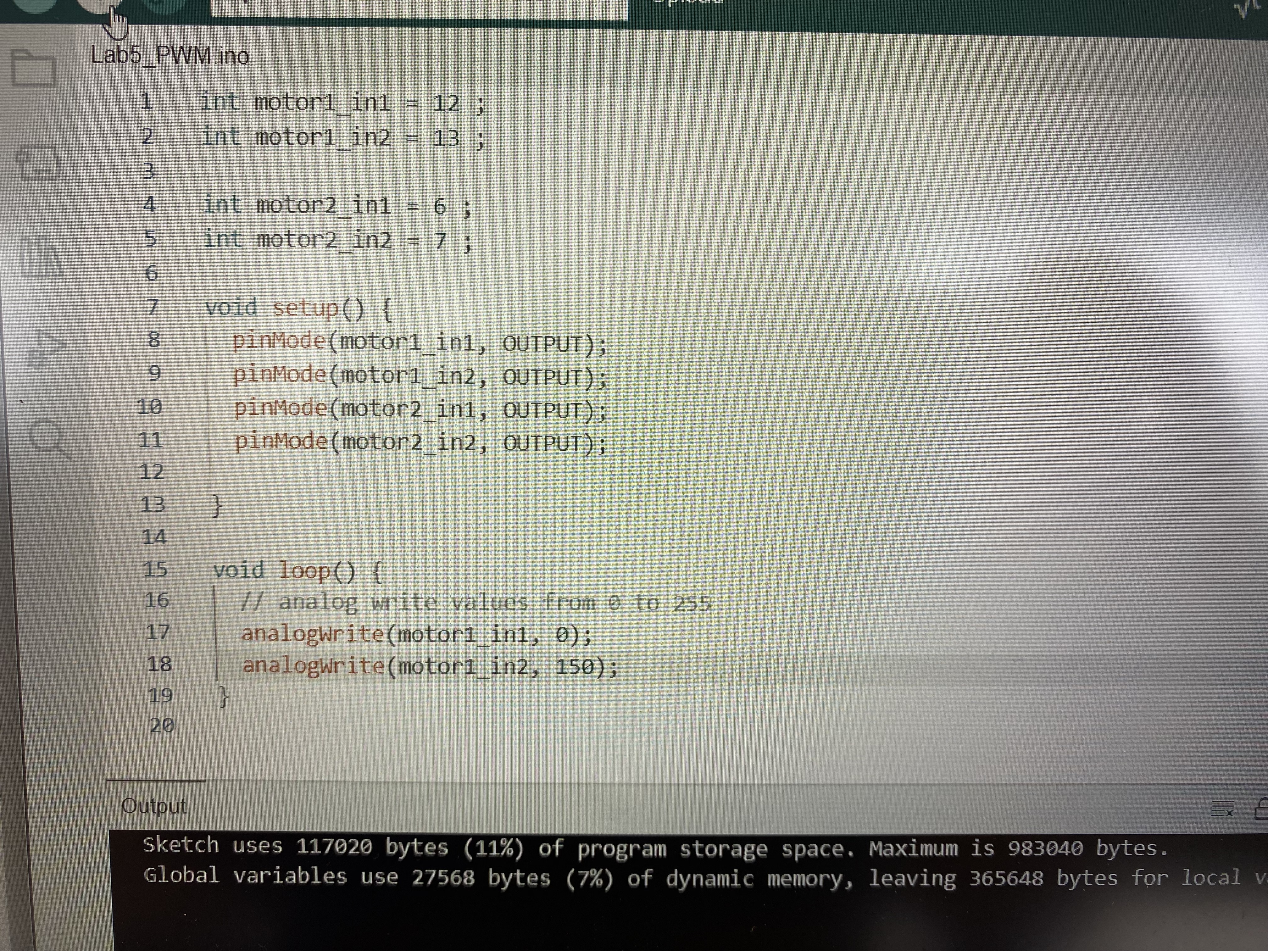
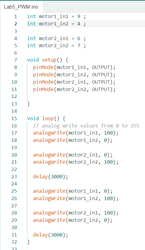
For motor control on the Artemis I ended up using pins 9 and 4 for the right motor
and pins 6 and 7 for the left motor. Originally I wanted to use pins 12 and 13 however,
after debugging it seemed there was an issue with sending signals from those pins.
Batteries
We power the the Artemis and the motors from separate batteries because they have different power requirements.
The Artemis is powered by the 3.7V 650mAh battery. Whearas the motors are powered by the 3.7V 80mAh battery.
The motors use up a lot of power/current which is the reason we should power them with a separate battery.
Lab Tasks
Soldering Motor Drivers
I soldered both motor drivers at the same time so I didn't have to
do all the work for one and then repeat the process for the other.
I connected the inputs and outputs of A to B the dual motor drivers by looping the wire between the pins and
using either heatshrink and solder to connect them in place.
I also soldered wires for VIN and both GNDs (one to connect to the Artemis and the other to connect to the battery).
I ended up using solid core wires which might be a problem for later labs if I have to do repairs.
I didn't think about using the stranded wires until after I finished soldering both of my motor drivers.
One pro to using the solid core wires is that the motor drivers kinda just float in the air.
The con to using solid-core wires is that they might break during some of the high acceleration tricks.
But I guess I'll have to deal with the consequences in the following labs.
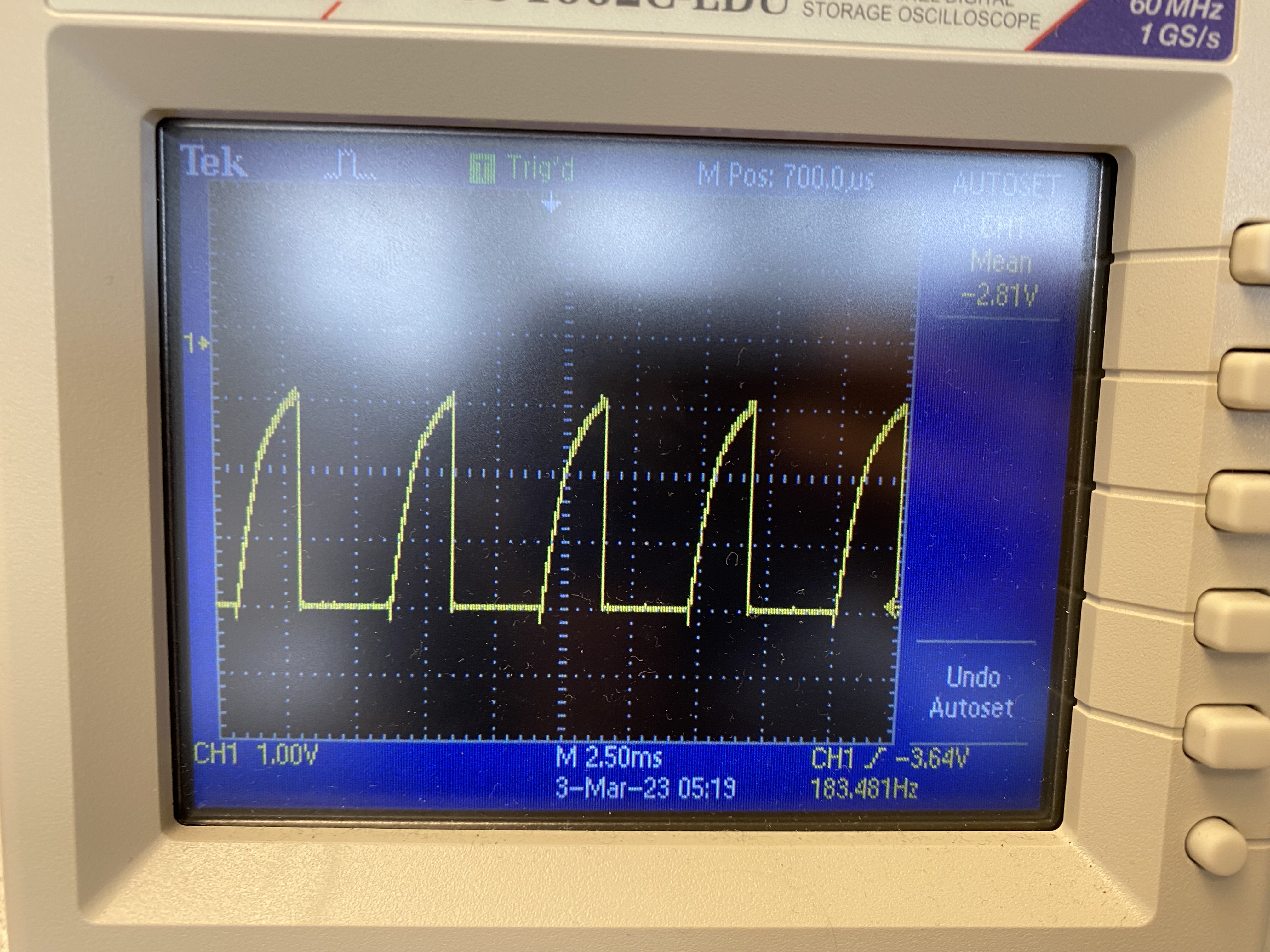
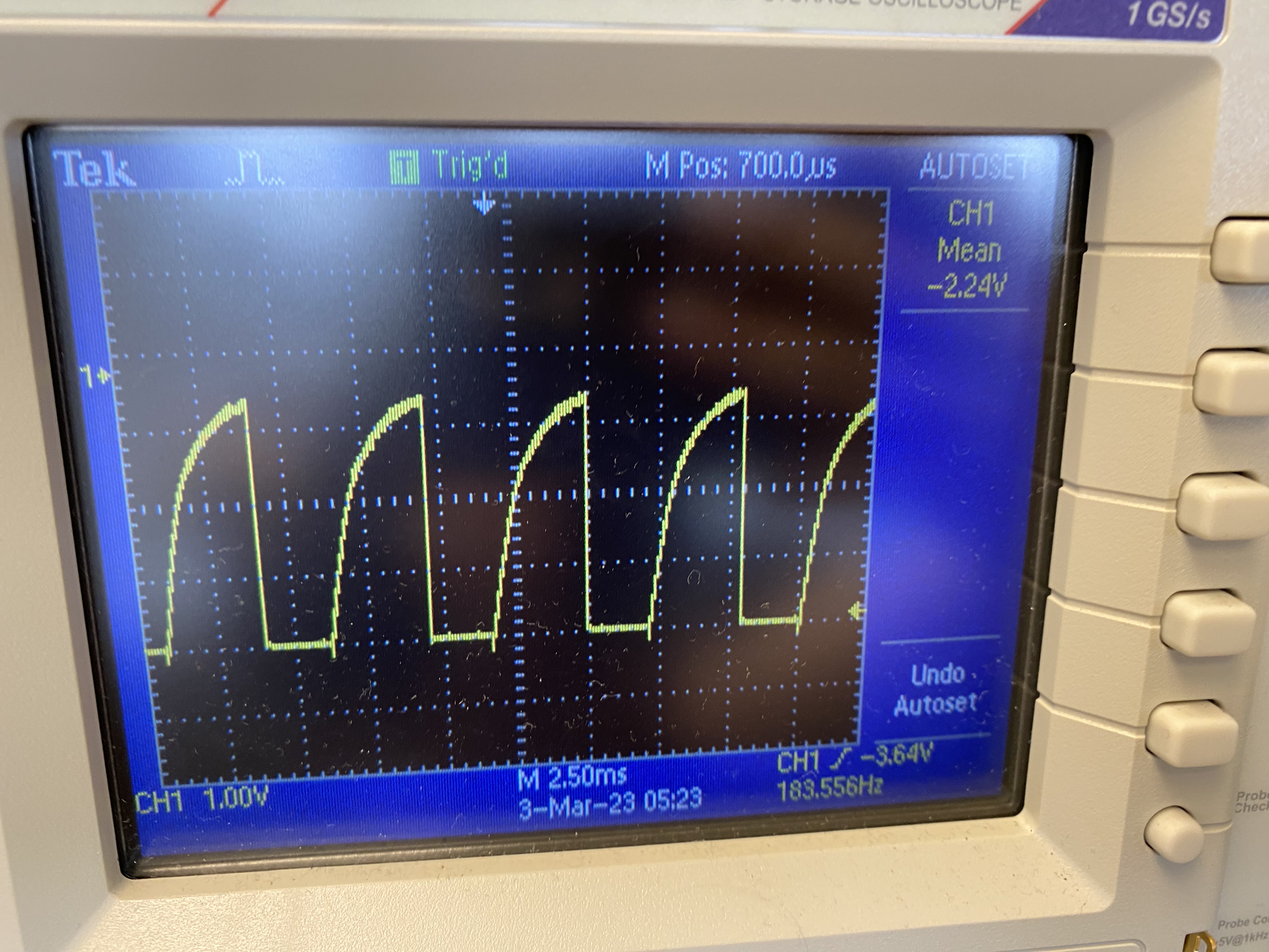
PWM Signals from Artemis
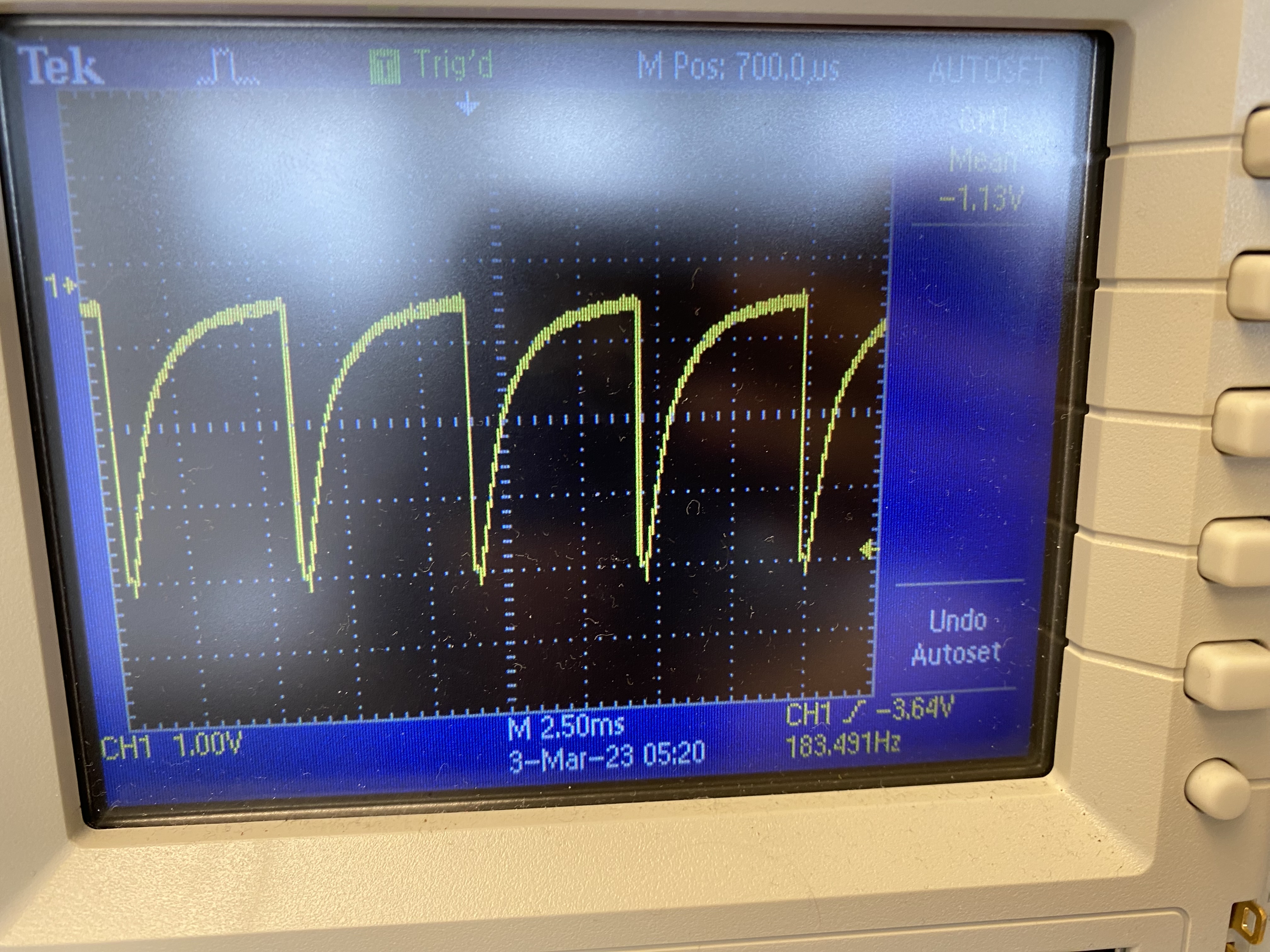
I used the oscilloscope to display the motor driver outputs as I used analogWrite (values range from 0 to 255)
to generate a PWM input from the Artemis. I kept one input at 0 and then adjusting the other input
to be a value between 0 and 255.
Below are some of the PWM values I tested with their scope:
Value 150:
Value 100:
Value 10:
Testing One Dual Motor Drivers with PWM Inputs
When testing one dual motor driver, I used an external power supply that hand
an output voltage of 3.7V since when the car is running the battery we will use
will be 3.7V 850mAh.
I continued to use the oscilloscope to display the motor driver outputs.
To change the direction of the motor (clockwise or counterclockwise) I switched
the inputs for the one that is set to 0 and the one I was adjusting. If I wanted the motor to stop, both inputs
were set to 0.
Below is a video of the left set of motors rotating and the video of the oscilloscope scoping the outputs.
Below is a video of the right set of motors rotating and the video of the oscilloscope scoping the outputs.
Test Both Dual Motor Drivers at the same time
Afterwards, I attached the motor driver to be powered by the battery and tested if both motors could run at the same time.
First I had both motors rotate in the clockwise direction (one forward, one backward) and then afterwards I changed the PWM input
for both motors to rotate in the forward direction and the backwards direction.
One interesting issue I ran into was that the motors works fine when running them on their own and in opposite directions at the same time.
However, when I tried to run them both in the forward direction my left motor did not spin. I debugged with the oscilloscope and the inputs to
the motor driver from the Artemis did not appear as desired. I ended up resoldering the motor driver inputs from pins 12 and 13 to pins 9 and 4.
Below is a video of the motors turning at the same time:
Pics of My Finished Car
I was able to attached everything to the car by using electrical tape. The motor drivers ended up floating in the air.
Running on Ground
I tried running the car directly on the ground. In order to make it easier to send different PWM values to the motors,
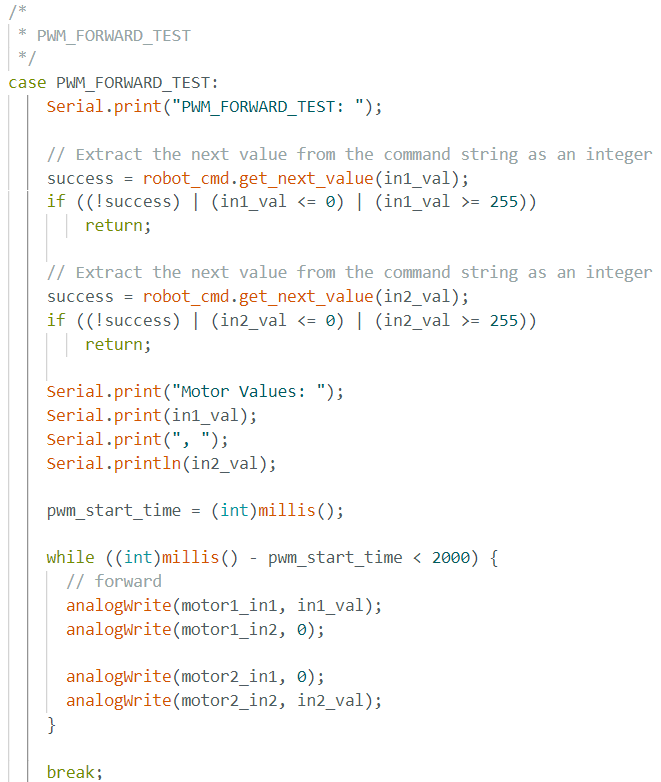
I created a new command in ble_arduino to take in two inputs (one for each motor) and then run for a short period of time before stopping.
The reason for using bluetooth is that I didn't want to continue compiling and burning code onto the Artemis if I only how to change a couple of values.
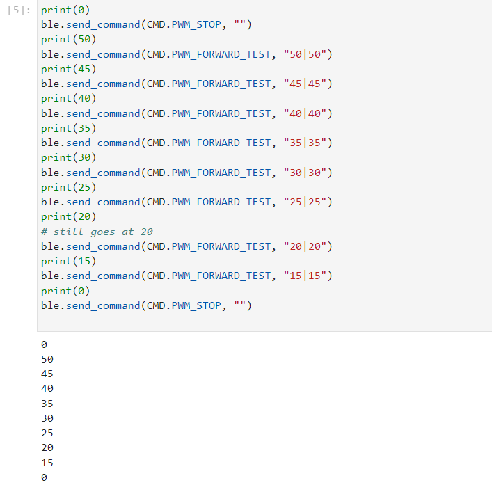
Lower PWM Limit
To find the lower PWM value that the robot could move on the ground when starting from rest and when already in motion.
After sending a variety of values to the robot, the lower PWM value to start the robot from rest is around 30.
To find the lower PWM value that allows for the robot to move on when already running, I input different values starting from
50 and decrementing by intervals fo 5 until a value of 15. I also printed which value I was inputing so I could watch when the
robot slows down and stops. It turned out the lower PWM value for when the robot is already running is around 20.
Calibration Factor
For the calibration factor, I just played around with different input values on both motors until the car moved in a fairly straight line.
My input values were 70 for the right motor and 50 for the left motor.
Open Loop
I made a separate command for my open loop demonstration. Within the command in Arduino I added a series of different movements.
Going straight, spinning clockwise, going backwards, and spinning counter-clockwise.
Lab 6: PID speed control
Objective
The purpose of lab 6 was to become familiar with using PID control. It is one part of a series of labs
dealing with PID control, sensor fusion, and stunts. We were given the option of doing
position control or orientation control, I chose position control. We also had to choose a controller
that would work best for our system, I chose PID.
Prelab
For the prelab we had to establish a good system for debugging the rest of the lab. I made a copy of my bluetooth code
from the previous labs and cleaned it up to only have a few command for this lab.
I planned to use two bluetooth commands to communicate between my laptop and the Artemis.
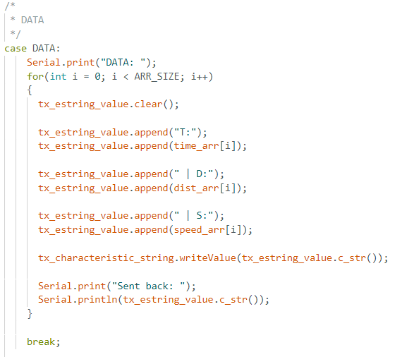
One command takes in the sensor measurements, controls the robot, and stores
the data in arrays. The other command sends the data that was stored in the arrays over bluetooth to my laptop in python. Since I knew
I wanted to do position control which only requires me to save data about the time, TOF sensors, and motor speed. On the python side,
I saved the arrays of data into pickle files so I could access the data to later on make graphs and for lab 7.
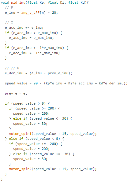
Task A: Position Control
Implementing PID
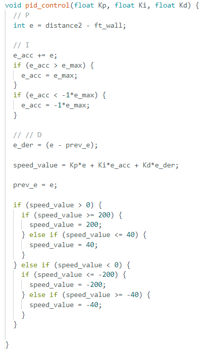
At first I wasn't sure which controller I was going to use so I just implemented PID and planned to
incrementally pick the coefficients based on my results using the robot. The error was based on
how the difference betweeen the tof sensor reading and 1ft (304mm) since the robot needed to stop
about 1 ft away from the wall. I also had to adjust if the robot would go forward or backward
depending on the error. I based my implementation on the slides provided to use in lecture and
also the implementation of PID from a class (ECE 4760 - Design Microcontrollers) that I took last
semester. The motor values are from 0-255 but as in the previous lab I found the lower PWM value to
be around 30. However, I redid this and set the minmum value to 40 and then set the max value to 200.
Process
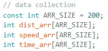
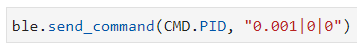
My bluetooth command allows me to input the kp, ki, and kd, values so I can quickly test out different
values without having to edit the arduino code. My arrays had a size of about 200 and the motors had an
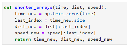
automatic stop after running for 15sec. Some of the values in the array ended up being 0 so I made a function
to get rid of the extra zeros that did not contribute to the data.
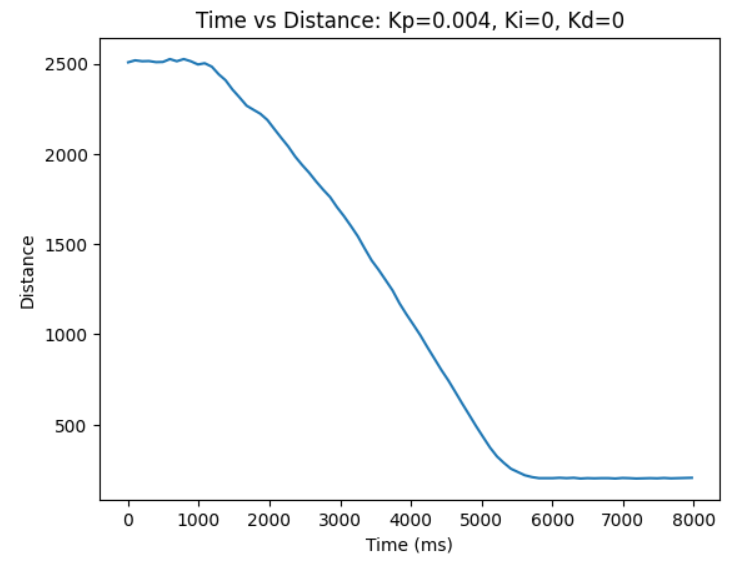
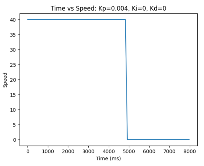
I followed heuristic procedure #2 when deciding on the values. I set ki and kd to zero
and adjusted the kp value. I started at a very small kp value (0.001)
and increased the values until the robot stopped around 1ft away from the wall. The kp value was set to 0.004.
Then I decrease the kp value by a factor of 2-4 and slowly increased ki until there was a loss of stability.
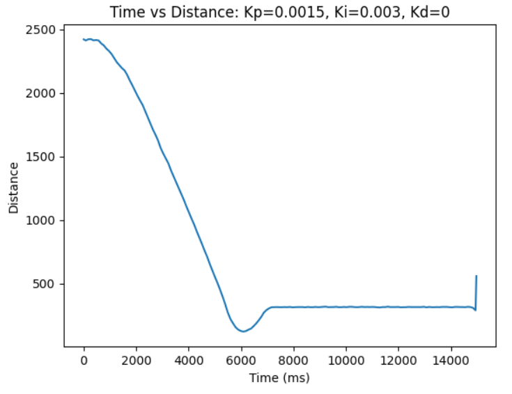
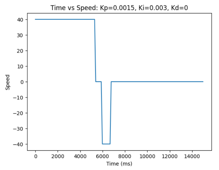
The kp value was set to 0.0015 and the ki value was set to 0.003. As you can see the robot goes passed the
1ft mark but moved backwards to the proper position.
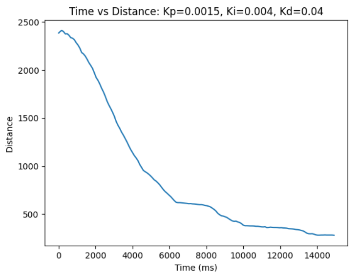
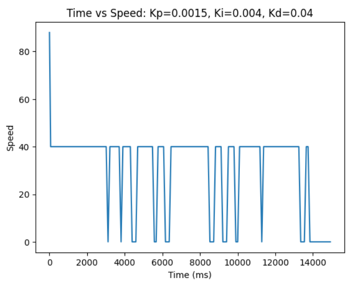
Then I added the kd value and increased it until there was some sort of response to the disturbance.
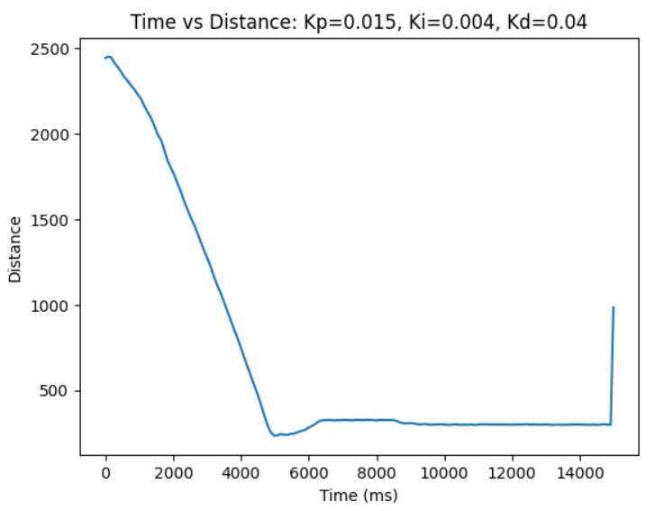
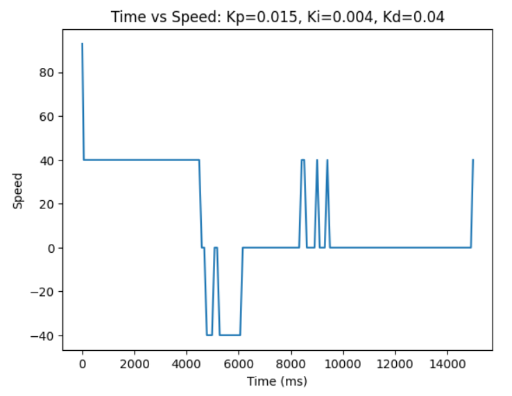
The kp value was set to 0.0015, ki set to 0.004, and kd was set to 0.04.
The robot kept stopping so I decided to increase the kp value to 0.015.
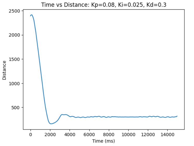
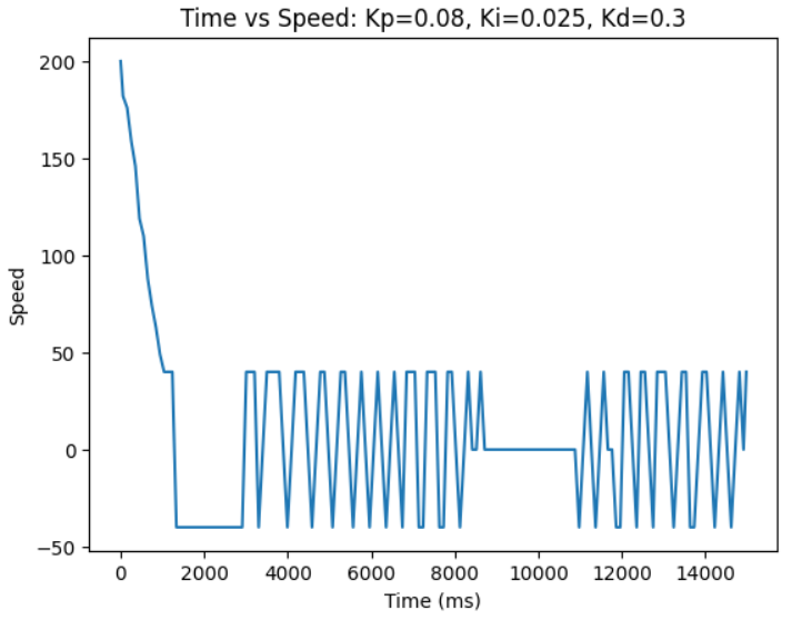
Afterwards I was talking to another classmate and they recommended using a high kp and kd value.
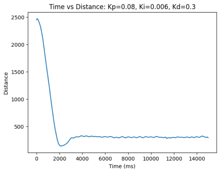
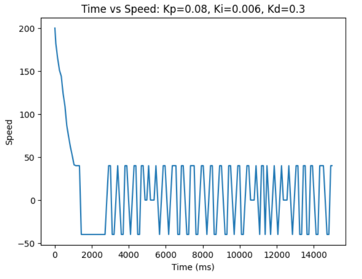
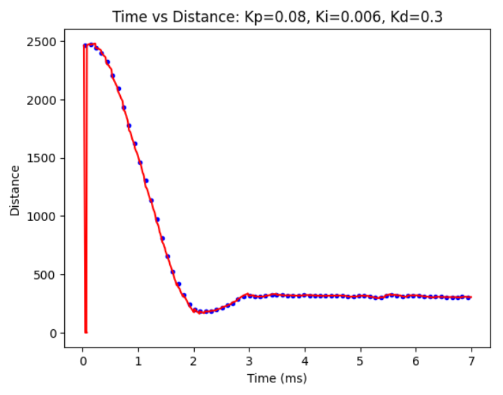
The robot went way faster then before. The values used below were kp = 0.08, ki = 0.025, and kd = 0.3.
I played around with the values some more and ended up with
kp = 0.08, ki = 0.006, and kd = 0.3.
Resources
I used my PID implementation from ECE 4760. I also spoke with Liam Kain about increasing the
kp and ki values to make the robot fast.
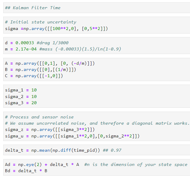
Lab 7: Kalman Filters (sensor fusion)
Objective
The purpose of lab 7 was to implement the Kalman Filter to help execute
the task from lab 6 at a much faster speed. First we implemented the Kalman
Filer in python. For the last part of the lab we were supposed to implement
the Kalman Filter directly on the robot however, due to the Snow Day we were
given the option to just extrapolate the next position based on the most recent time-of-flight
data point.
Lab Tasks
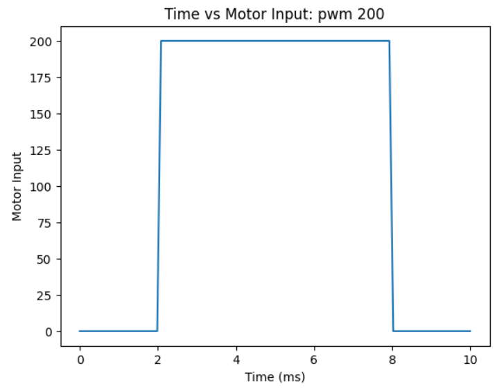
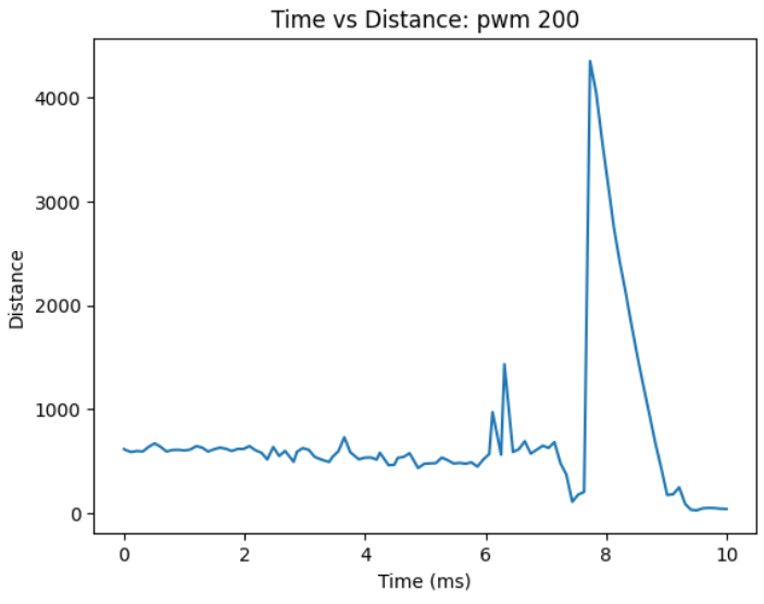
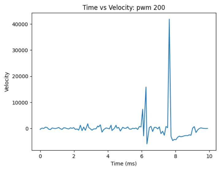
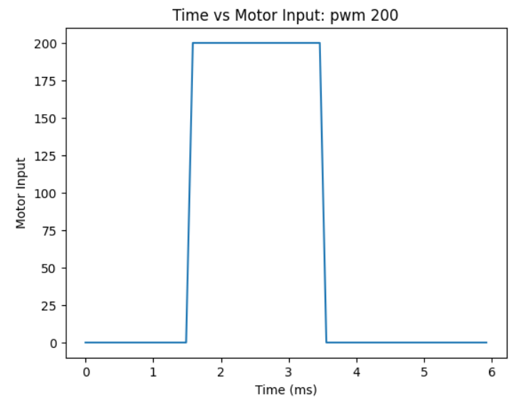
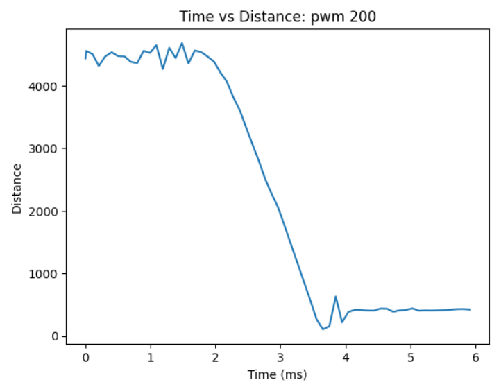
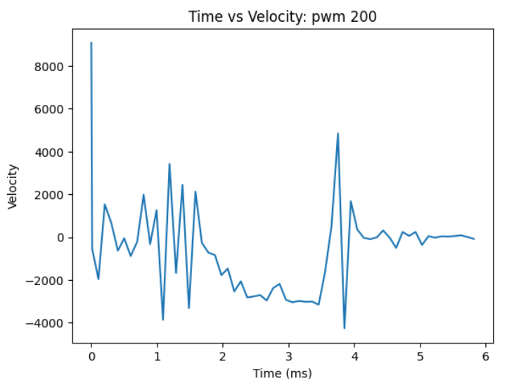
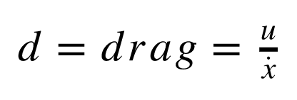
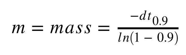
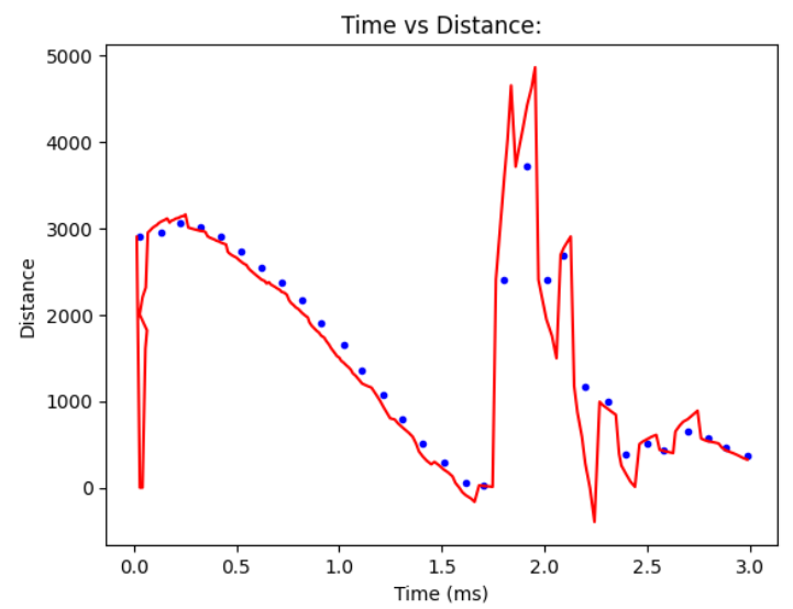
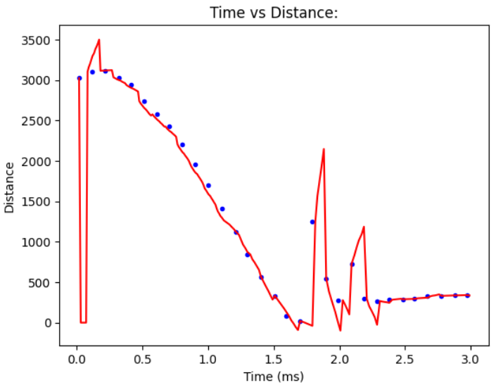
Task 1: Estimate Drag and Momentum
To estimate the drag and momentum, I used a step response to gather
information about the motor input values and ToF sensor output.
Based on the last trial of my lab 6, I chose the PWM value of my motor to be 200.
In order to find the steady state velocity and the 90% rise time to get to the steady
state velocity, I had to do two different runs. The first run was starting the robot
from over 4.5m (out of range for the ToF sensors) so I could see what the steady state
velocity was. The second one was from less than 4.5m so I could properly see the
value of the 90% rise time.
Starting Robot from over 4.5m (begins out of range for ToF sensors)
Starting Robot from less than 4.5m
Based on these trials the steady state speed is 3000mm/s and 90% rise time was 1.5s.
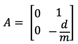
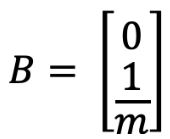
Task 2: Initialize KF
The steady state speed was used to calculate the drag and u was set to be 1. The drag
was calculated to be 0.00033. The drag and 90% rise time were used to calculate m to be
2.17*10^-4.
The drag and mass were then used to compute the A and B matrix.
The C matrix was provided to us in lecture: C = [-1 0].
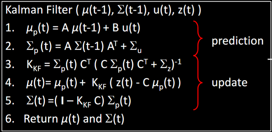
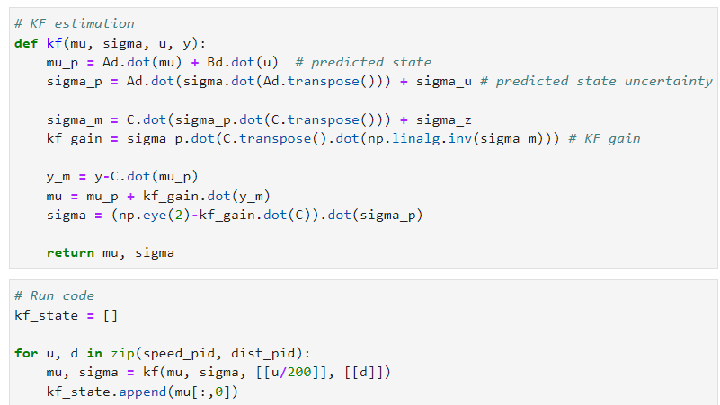
Task 3: Implement and test Kalman Filter in Jupyter
I mainly followed the steps and code provided to us in lecture for implementing the Kalman Filter.
I played around with the sigma value to put more confidence either in the model or in the data points.
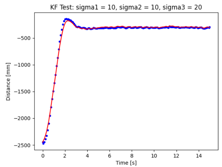
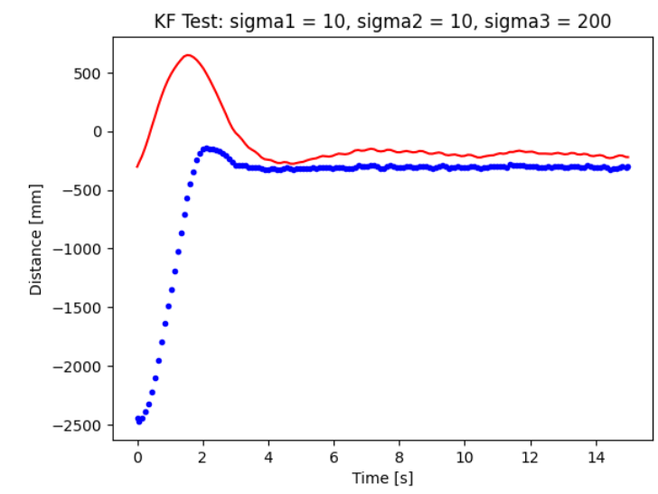
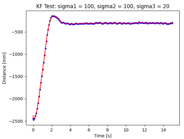
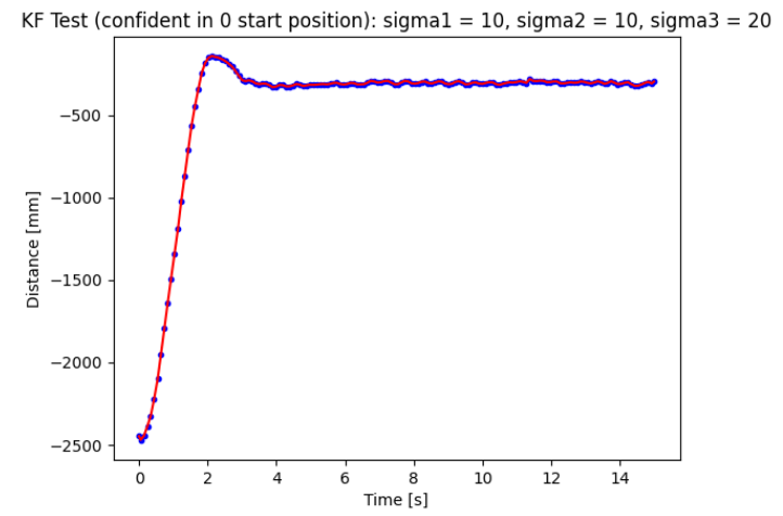
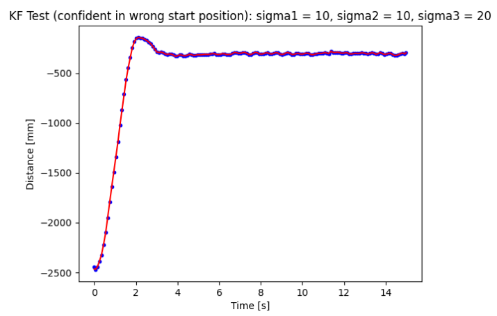
To start off I set sigma_1 = 10, sigma_2 = 10, and sigma_3 = 20.
The orginal sigma values:
Changing the sigma values to put more trust on the model:
Changing the sigma values to put more trust into the TOF sensor data:
Original sigma values: Confident in starting position
Original sigma values: Confident in starting position that is off by 500 mm
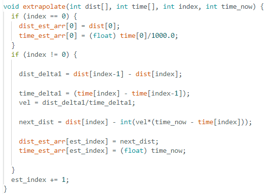
Task 4A: Extrapolation
I extrapolated the values based on the ToF sensors. I made a separate function to calculate
the extrapolated values and stored them in a separate array. At first I didn't realized we were
just seeing how well our model followed the senor data. I thought we had to use our extrapolator
to control our motors but that will happen in lab 8.
Resources
I looked at Anya's website from last year. Liam Kain also helped me debug my extrapolator since it was
hard faulting due to the arrays of the estimations not being big enough.
Lab 8: Stunts
Objective
The purpose of this lab was to combine all the work we did to a fast stunt. Since I
chose Task A: Position Control in lab 6, the stunt I completed was to quickly drive the robot
from the designated start line, flip when reaching the sticky mat, and drive back from where it came.
Lab Procedure
Stunt Set-up
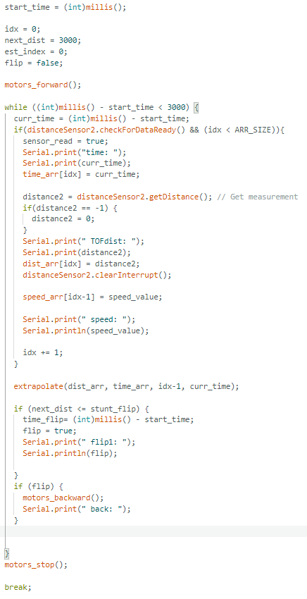
I edited my lab 7 code by deleting the pid control and using my extrapolator quickly calculate the
distance from the robot to the wall. Once the robot gets within the range of the sticky mat it changes
direction from forwards to backwards to initiate the flip.
Edited Code:
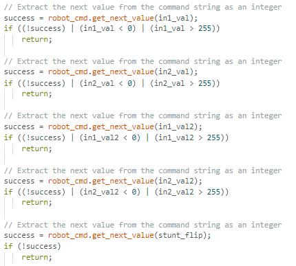
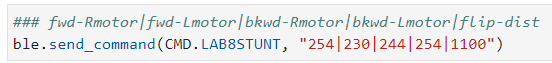
I also ended up adding command inputs for the pwm values for each motor in the forward and
backward direction as well as the desired flip distance from the wall.
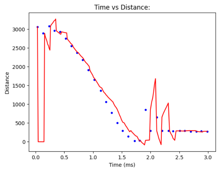
Trials and Errors
I took many different trials in the hallway of Phillips Hall. As shown in the videos below there was much variety to
how the robot interacted in the hallway which lead to me getting closer to completing the stunt.
This allowed me to see that the robot is about to go forward in a straight line and is able to reverse direction when it
gets to the specified distance from the wall. The issue here was that the motors were not fast enough to flip it over but
it was able to angle the robot in a different direction. I increased the motor input values but still tried to maintain the
straightness of robot which led to me having values of 250 and 192.
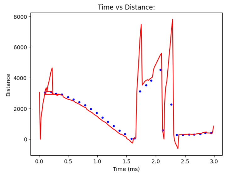
The robot's behavior is similar to the previous video however, it is able to lift partially off the ground. I need to increase
the PWM values for the robot in the backwards direction.
Then the robot was able to flip but it ends up rotating away from where it came from. Liam recommended slightly angling the
robot to account for the robots rotation during the turn. Then I was able to get actual trials for the robot. Yay!
Stunts
Trial 1
Trial 2
Trial 3
Trial 4
Cool Move for Fun
Resources
Liam Kain helped me with some of the debugging for how to angle the robot to make it go forward and
return to the starting line.
Lab 9: Mapping (real)
Objective
The purpose of lab 9 is to map out the set-up in the lab room using
distance sensors collected from the ToF sensors and angle measurements from the gyroscope.
There are five points throughout the map (-3, -2), (0, 0), (0, 3), (5, -3), and (5, 3) for us
to place our robot and collect the measurements. We can chose from one of three options for how we want
to obtain these measurements which could be either open loop control, PID controol on orientation,
or PID control on angular speed. I decided to use the third option of PID control on angular speed.
After collecting all of our data, we use transformation matricies to combine and plot all the points on
the same graph. And then drawing the map using straight line segments.
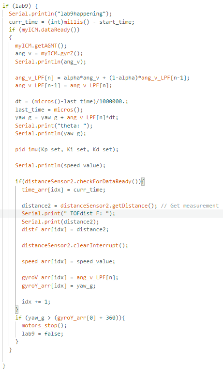
Lab Tasks
Angular Speed Control
When using angular speed control, the lab instructions recommend it is based on
an angular speed of a maximum of 25 degrees per second to allow for about 14 sensor readings spaced out at approximately
1s. I ended up basing my PID control on about 20 degrees per second. This gave me somewhere between
150 to 158 sensor readings. The PID control is based on the PID function I made for Lab 6 and was adjusted
to work for raw data from the gyroscope.
At first I wanted to use both ToF sensors to collect data but my sensor on the side of the robot was not working properly.
Therefore, I only collected data with my front ToF sensor. I calculated the degree measurements by using a
low pass filter on the angular velocity (degrees/s) from the gyroscope and then multiplying it by the time difference.
I stored the time, angle (degrees), distance (mm), angular velocity (deg/s) and motor input into arrays that I could send over
to my python script. In addition, to make sure the robot car stopped turning after spinning 360 degrees I checked if the yaw value that
was being read from the gyroscope was greater than 360.
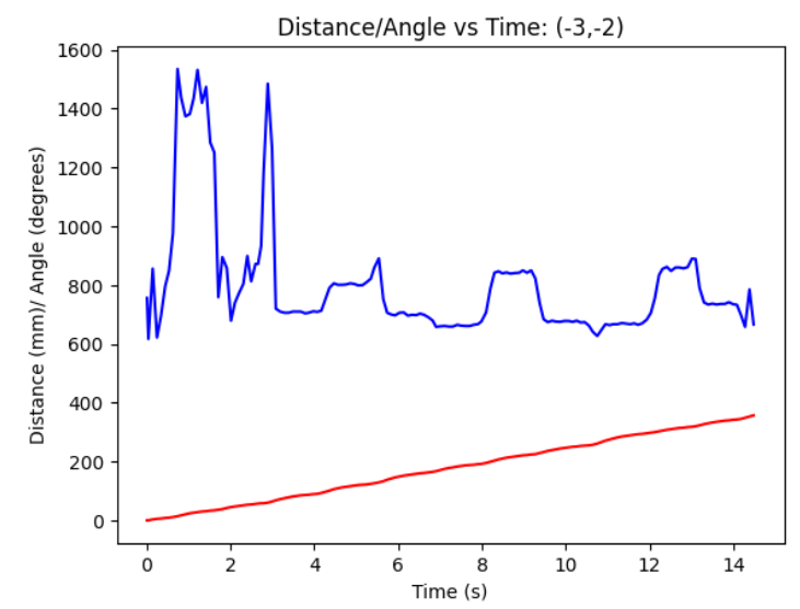
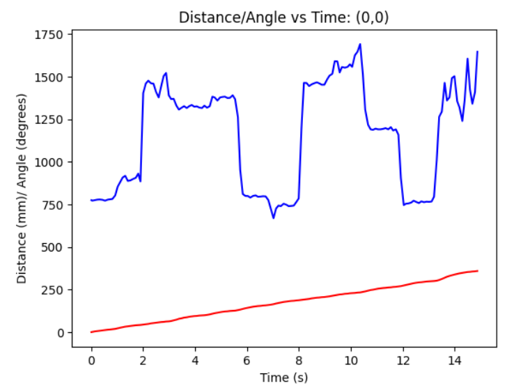
This is a video of the robot in action at the point (-5, 3). As you can see the spin is not very smooth which is due to me not
adjusting my Kp and Ki values enough. I settled with Kp = 0.35 and Ki = 0.6. On the bright side the robot was able to stay somewhat
centered while spinning. In the future, I would want to improve and perfect the spin. (when looking at the data measurements you can
see how the abrupt movements may have affected the readings)
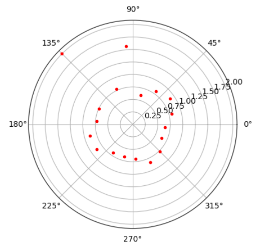
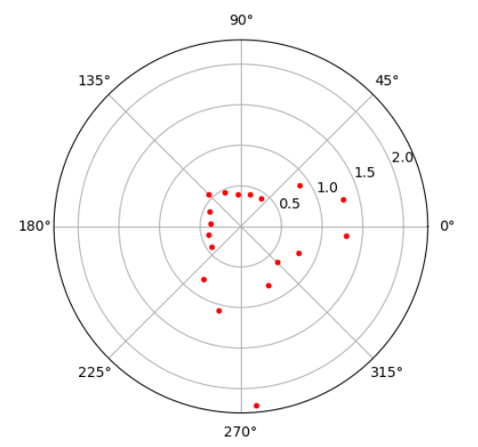
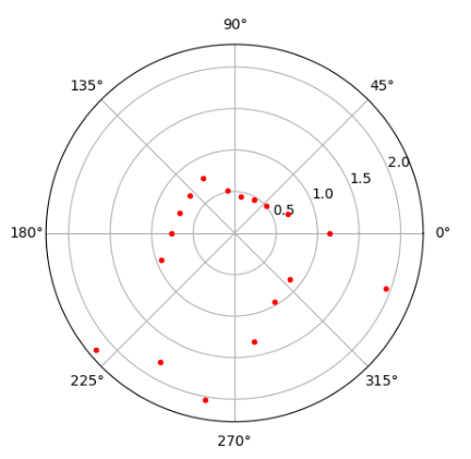
Reading out Distances
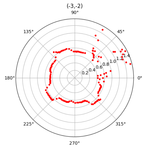
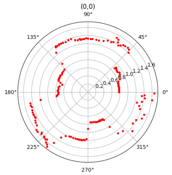
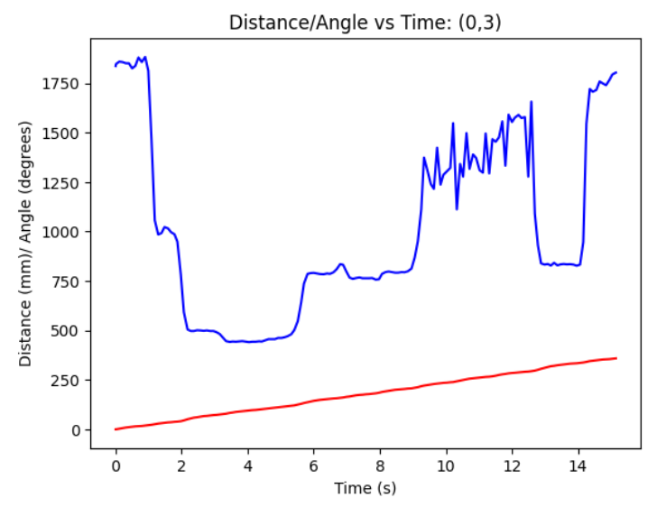
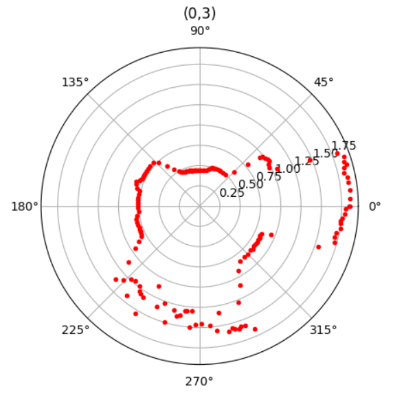
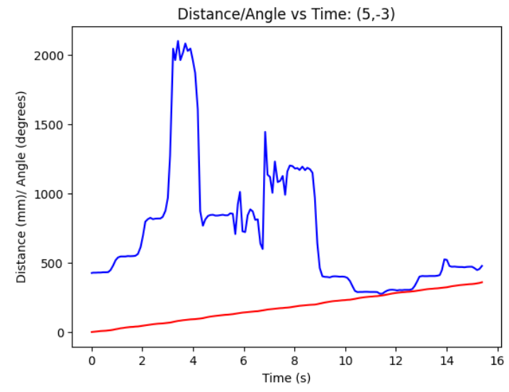
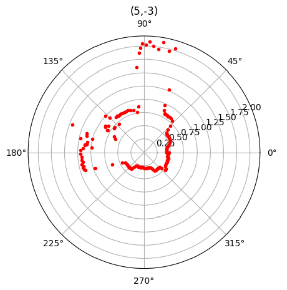
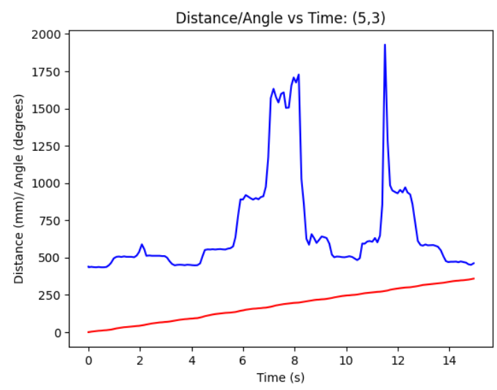
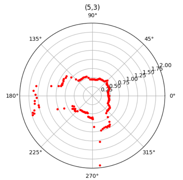
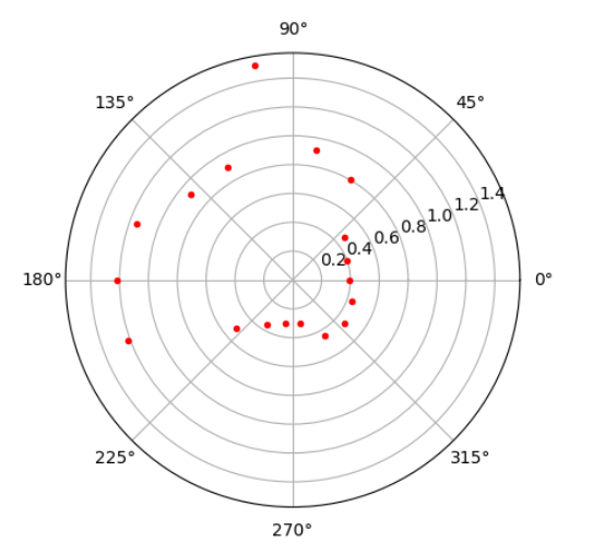
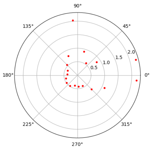
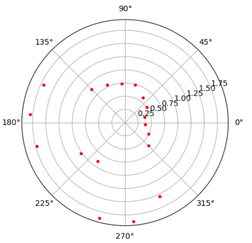
I placed the robot at all 5 points on the in-room map and plotted the distance and angle readings.
One thing I did not notice at first was how the polar plot takes in the angle as radians but after this
quick fix I was able to see if the plots matched what I saw in real life. In addition, I started the robot
with the ToF sensor facing the right side of the room since that is where 0 degrees faces and I didn't have to
rotate my data when later on merging the plots.
(-3, -2)
(0, 0)
(0, 3)
(5, -3)
(5, 3)
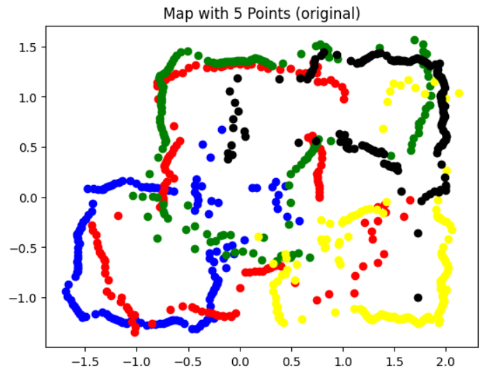
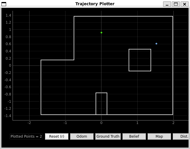
Merge and Plot Readings + Line Based Map
To merge all the plots into one I ended up following Ryan Chan's transformation matricies code from last year.
The original plot shows the general layout of the room. There are many points and it it not very smooth which
could be due to the turn have a stop/go motion. I would say it's not terrible but definitly has room for improvement.
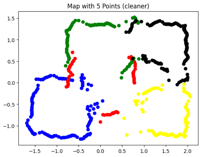
Afterwards, I filtered out some of the outliers (based on Tiffany Guo) to get a cleaner plot.
Then, I added the line-based map to the plot
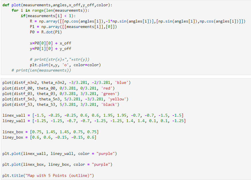
Here is the python code that was used to create the Merged Plots and Line Based Map:
Resources
I looked over Anya and Ryan's websites from last year. I also referenced Tiffany's website. As well as received
advice from Zin for how to orient the robot when collecting the data for the plot.
Lab 10: Localization (sim)
Objective
The purpoes of lab 10 is to implement grid localization using Bayes filter
on the robot simulator. This is to prepare us for what to expect in the next lab where we will
use localization on our actual robot.
Prelab
Prelab
For the pre-lab we read through background information about
localization, sensor model, motion model, and Bayes Filter Algorithm.
This was so we could be prepared to implement everything in python.
The purpose of localization is to determine where the robot is located based on it's
environment.
Lab Tasks
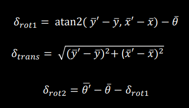
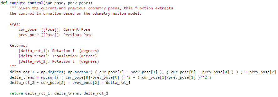
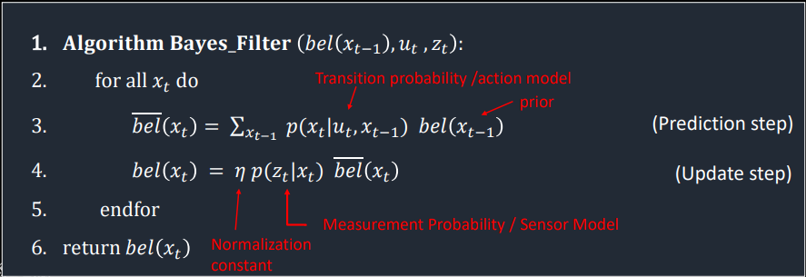
Compute Control
The compute control helper function computes the control variables delta_rot1, delta_trans, and
delta_rot2 based on the current and previous position from the odometry model. The code is based on
using the delta_rot1, delta_trans, and delta_rot2 equations from class.
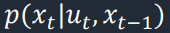
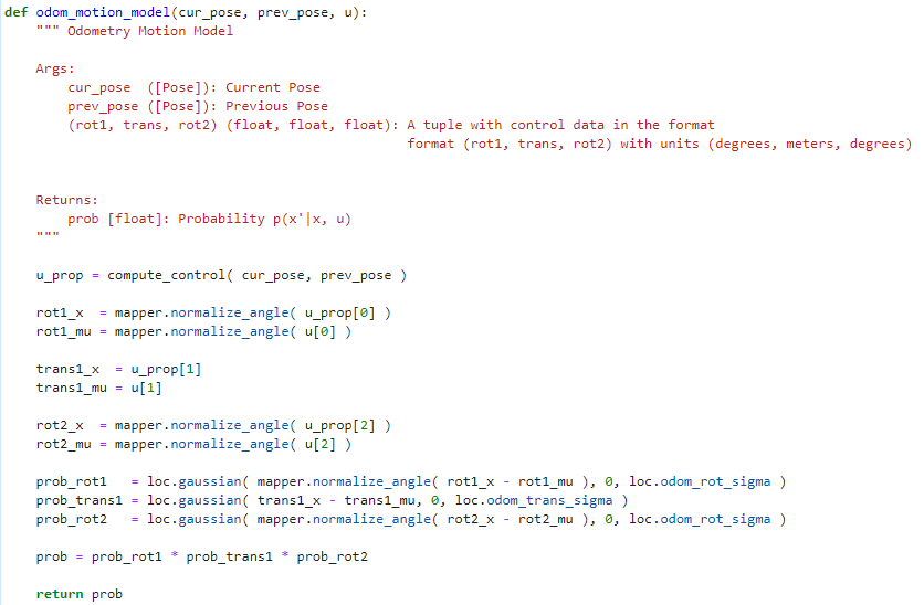
Odometry Motion Model
The Odometry motion model takes into account your current position, previous position,
and where the robot was supposed to be to compute the probability of where the robot
was expected to be versus where it actually is. This is done by using compute control
to get the control information based on the provided current position and previous position
then normalizing all the values of rotation1, translation1, and rotation2. Afterwards,
the probability is computed for each of these values by using the gaussian distribution on
difference between the actual and expected control variables with their respective sigmas.
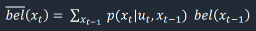
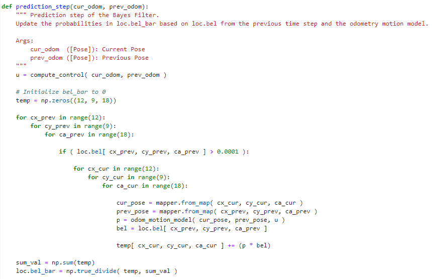
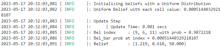
Prediction Step
This is the prediction step of the Bayes Filter which updates the probabilites in the matrix
bel_bar which is the prior belief before the latest measurement. The code loops through
the previous and current x, y, and rotation values to calculate the current position, previous
position, the odometry model, and the belief based on the previous x, y, and rotation
values. For this implementation, if the belief of the previou values is less than 0.0001
the next calculations are not done to mitigate the computational load. From here the summation of the product of odometry motion model and the belief
is calculated. Then, the numbers are added together and normalize to return the prior belief.
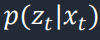
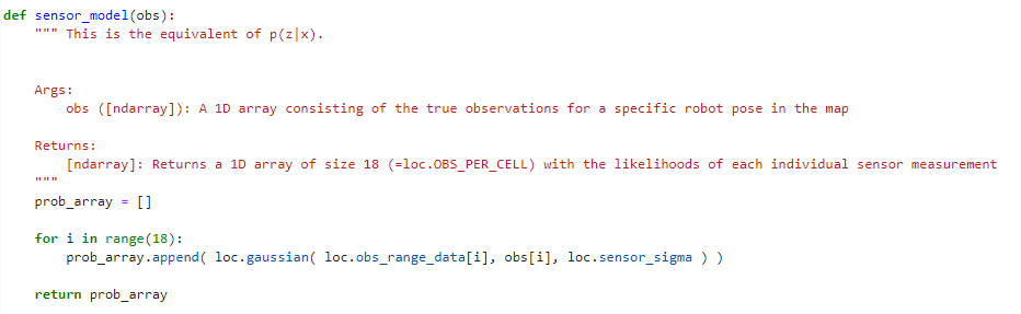
Sensor Model
The sensor model is similar to the odometry model however, this function uses the gaussian distribution
to calculate the likelihoods the each individual sensor measurement based on the data collected by the
robot and the sensor sigma.
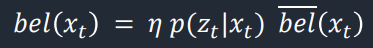
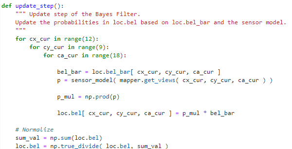
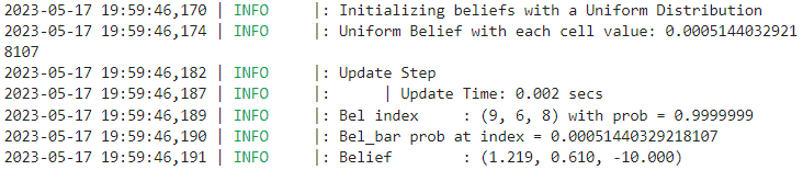
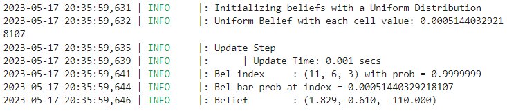
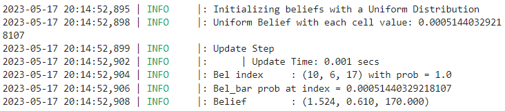
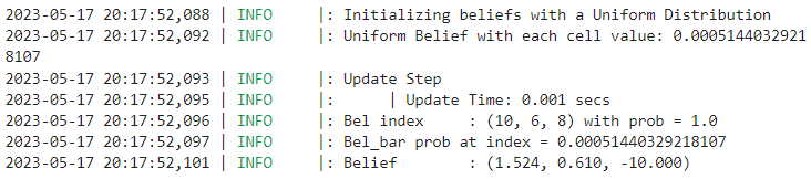
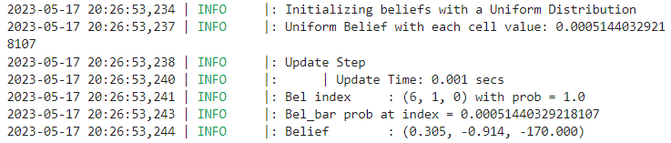
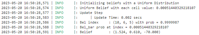
Update Step
This is the update step of the Bayes Filter which returns the belief of the robot based on all
the past sensor measurements and controls. It loops through the current x, y, and rotation values
to calculate the prior belief, sensor model, the product of the vales in the sensor model probability
array. Then the belief is calculated by multiplying the product of the sensor model values by
the prior belief. Then this is normalized.
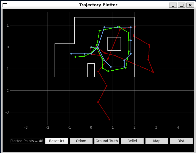
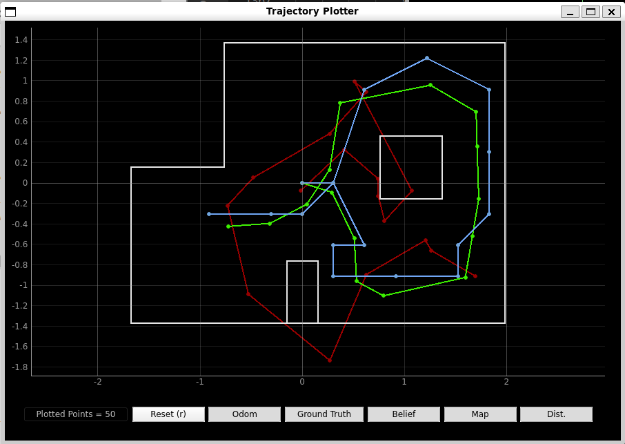
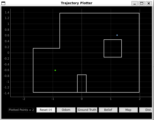
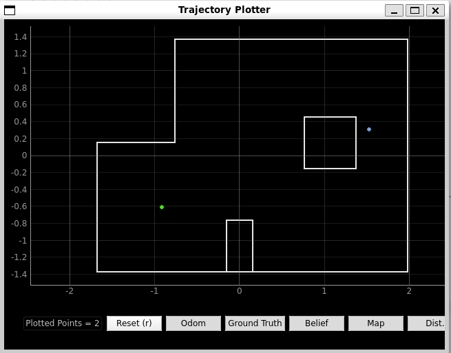
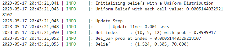
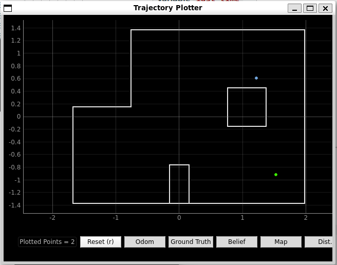
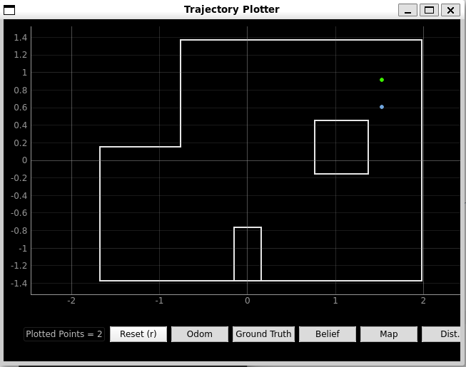
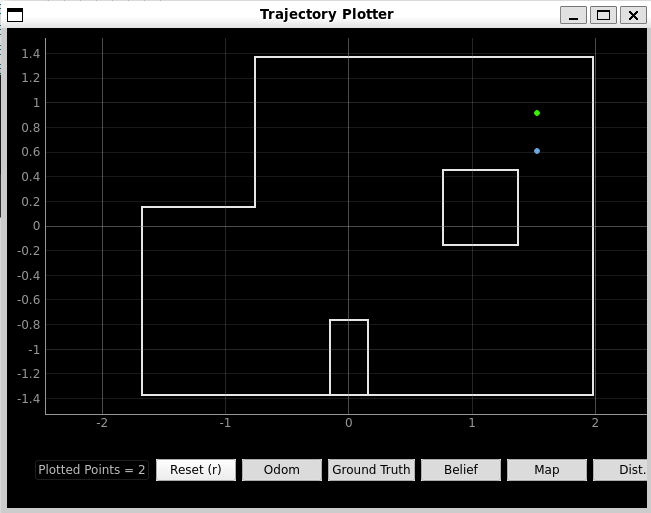
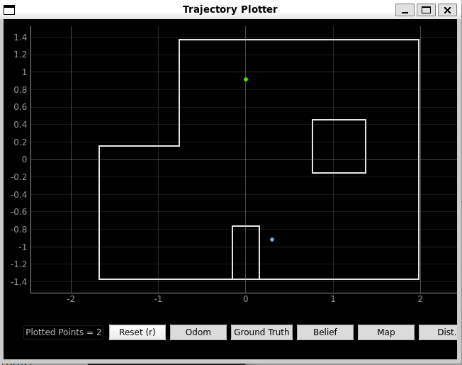
Bayes Filter Algorithm Running
I ran the Bayes filter. The green line represents the ground truth, the red line is odometry, and the blue line is
the Bayes filter values. The Bayes filter values seem to follow the ground truth pretty closely. It's not exactly
the same but the general shape is similar and there is not much error. The odometry model on the otherhand is very far off
from both the ground truth and odometry model.
Resources
I looked at Anya's code and website from last year as reference for this lab.
Lab 11: Localization (real)
Objective
The purpose of this lab is to perform the Bayes filter on the robot
in real life.
Pre-lab
For the pre-lab we had to read through the lectures, grid localization, and other important
information on the lab 11 instructions page. We also had to set up the base code by
copying the lab11_sim.ipynb and lab11_real.ipynb files
Lab Tasks
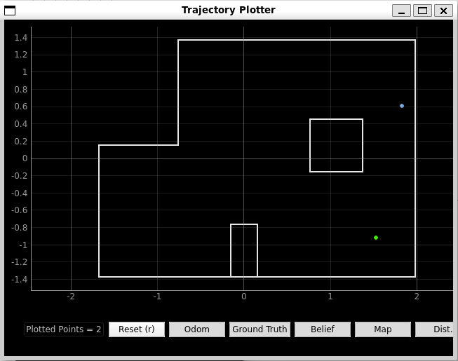
Localization in Simulation
First we tested the localization in the simulation from the notebook
lab11_sim.ipynb as shown below.
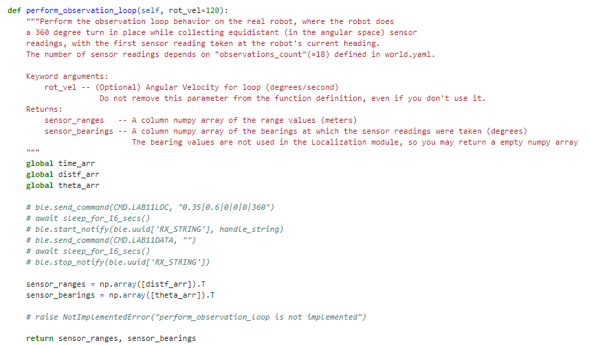
Perform Observation Loop
The robot need to output ToF sensor readings taken at 20 degree increments
starting from the robot's heading. I decided to edit my lab 9 code so instead
of collecting data for the full 360 degrees, it only collects it every 20 degrees.
This is done by keeping track of the current angle and the previous angle (a multiple of 20)
and checking if 20 degrees has past. I am also only storing the time, distance measurements
and angle measurements to send over to python.
On the python side, at first I was going to just call the ardiuno commands in the function
but after some failed localization (I forgot to save screenshots) I decided it would be
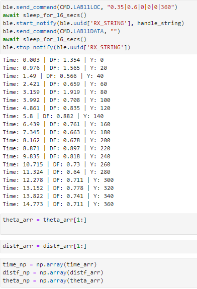
better to collect the data outside of the perform_observation_loop() function and just pass the function the arrays
of the 18 measurements. In the screenshot you can see an example of the data collected
when the robot ran at (-3, -2).
Collecting data
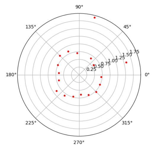
I collected data at each of the 4 points (-3, -2), (0, 3), (5, -3) and (5.3). I did two trials
for most of the points and compared the polar plots to where the simulator thought the robot was.
Most of the data that was collected you can tell it is similar to other points on the map which could
have lead to the inaccurate resutls.
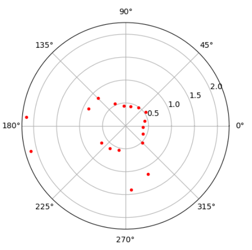
(-3, -2) Trial 1: Facing 270 degrees
(-3, -2) Trial 2: Facing 0 degrees
(5, -3) Trial 1: Facing 0 degrees
(5, -3) Trial 2: Facing 180 degrees
(5, 3) Trial 1: Facing 180 degrees
(5, 3) Trial 2: Facing 0 degrees
(0, 3) Trial 1: Facing 90 degrees
(0, 3) Trial 2: Facing 0 degrees
I was planning on going back in the lab to figure out how to improve collecting data. I think
the main problem right now is with the spin and how it stops about every 20 degrees (look at lab 9 for reference).
Once the spin is improved I think it would collect more accurate data since it does spin on an axis pretty well.
I was able to slightly improve the speed by adjusting the angular speed the pid was based on from
20 degrees/sec down to 10 degrees/sec. This causes the robot to move in increments of about 10 degrees.
The only problem is that the robot turns very slowly.
I also tried to adjust the KP, KI, and KD values and the reason for it to seemingly move in increments
is due to the values that were chosen. If I adjust the values more the robot does turn more smoothly
however, it does not stay consistantly on the axis. On the otherhand, if I keep my current values it does
move sort of on an axis but moves incrementally. This is something I will have to decide between.
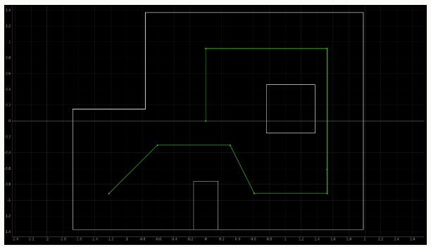
Lab 12: Planning and Execution (real)
Objective
The purpose of this lab was to use everything we implemented throughout the semester to have the
robot navigate through a set of waypoints as quickly and accurate as possible. It was up to each person to decide how they wanted to
have the robot navigate through the robot. Originally I was thinking of using Localization however, my lab 11 data did not go well and
I was running out of time to complete the labs.
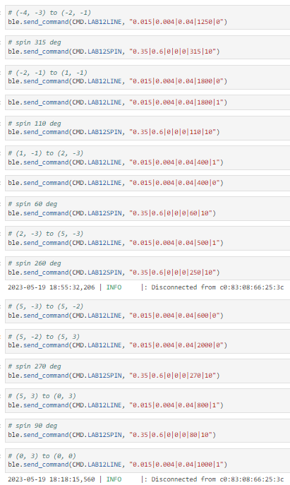
Therefore, I decided to use PID control for the angle measurements (lab 9) and the distance to stop (lab 6). Afterwards, I hardecoded
the distance and angle to move to each waypoint.
Lab Tasks
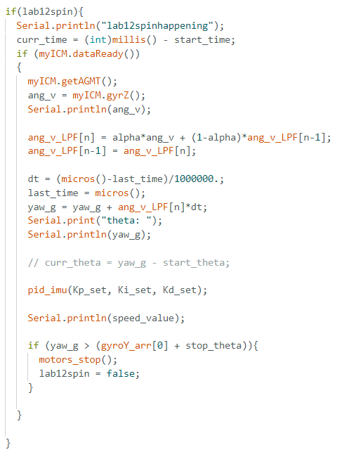
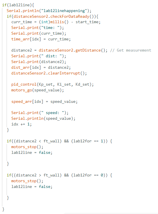
Arduino Code
I made two new case statments one for the spin and one for the distance movement. For the spin, I used similar code to what I had in
labs 9 and 11 expect I added another input parameter for how much the robot should spin at once. In addition, in order to make my spin more accurate
I also added a parameter for the angluar velocity that the PID was based on. I ended up having the PID be based on a 10 degrees/second angular velocity
so I could input smaller angle measuremnts for the robot to turn to. For the distance movement, I reused my code from lab 6 with certain kp=0.015, ki=0.004, kd=0.04 values
and when it reached a specified distance the robot will stop. I also added another parameter (1 to go forward and 0 to go backwards). I first tested all of these commands to
make sure the results were replicable.
Python Code
I ended up just hardcoding all of the movements with my PID commands. The main thing I had to consider what what direction I wanted my TOF sensor on the front to face.
I decided to sometimes have the robot movebackwards with the TOF sensor facing the wall it was closer to so it could accurately read the wall measurements.
This also meant I had to spin the robot multiple times when it was near the wall. Something I would improve is having the ability to have the robot spin both counter-clockwise
and clockwise since it was annoying to have the robot spin over 200 degrees. Also, my spin was very slow (360 degrees took about 30 seconds)
Video of Succesful Run
It was able to navigate properly through most of the waypoints except for the last one. It honestly went better than I expected. I think
the most important part was just having good PID control of the robot that allowed for accurate and consistant angles and distance stops.
Resources
I spoke to a couple of students about what their plan was for lab 12 and in the end I decided to go with PID control
to save some time.